How can I make a 2D line plot with a drop shadow under the line?

Question

You often see plots styled like this (ignore the bar chart component):

i.e. with a small drop shadow under the line. (I'm assuming Excel is being used to produce these plots).

How could you make something similar in Mathematica?

Answer 1

Here are some financial data:

data = FinancialData["GE", {2000, 1, 1}]

Hard-edge shadow

To make shadow put a slightly shifted down gray transparent copy of the curve under the original one. To make affect more subtle tune up Opacity[...] and other options. A small automation trick to answer @MikeHoneychurch comment - we use not a custom, but automated 0.1% of vertical width shift down. Other automation can be done (opacity, shadow width, etc), but I wanted to keep code simple.

DateListPlot[{{#[[1]], #[[2]] - .1 (Max[#] - Min[#])/100} & /@data,data}, 
Joined -> True,PlotStyle -> {Directive[Opacity[.4], Thickness[.01], Gray], 
Directive[Thickness[.004],Darker@Red]},AspectRatio->1/3, GridLines->Automatic]

Soft-edge shadow

Similar approach using Overlay and Blur. This makes shadow nicely soft.

a = DateListPlot[data, Joined -> True, PlotStyle -> Directive[Thickness[.004], 
Darker@Red], AspectRatio -> 1/3, GridLines -> Automatic, ImageSize -> 400];

b = Blur[DateListPlot[data, Joined -> True, PlotStyle -> Directive[
Opacity[.85], Thickness[.009], Gray], AspectRatio -> 1/3, Frame -> 
False, Axes -> False, ImageSize -> 380], 5];

Overlay[{b, a}, Alignment -> {.7, -.5}]

Answer 2

I'm sure there is a way of automating what I'm posting, but this can give you a general idea.

data = Table[{x, Sin[x] + RandomReal[]*0.2}, {x, 0, 2 Pi, Pi/50}];

g1 = ListPlot[data, Joined -> True, 
   PlotStyle -> {Thickness[0.01], RGBColor[0.7, 0.2, 0.2]}];

g2 = ListPlot[# + {+0.015, -0.015} & /@ data, Joined -> True, 
   PlotStyle -> {Thickness[0.01], RGBColor[0.7, 0.7, 0.7]}];

g3 = ListPlot[# + {+0.03, -0.03} & /@ data, Joined -> True, 
   PlotStyle -> {Thickness[0.01], RGBColor[0.9, 0.9, 0.9]}];

Show[g3, g2, g1]

Edit by halirutan: My answer would have based on the same idea, so instead of writing one myself, let me point out, what makes this approach IMO so nice looking. It is the effect, of having not a hard shadow, but a shadow where the edges are smoothed out. In reality there are rarely situations, where you have really hard edged black shadows and therefore a decent, slightly blurred shadow looks in graphs very nice too.

There are some free parameters, for instance the shadow position, its darkness, the grade of the blurring. If I would have to write a function, which does the same what is shown above, I would maybe use a Table, to create plots of the data with decreasing thickness and increasing darkness. Combining them gives a shadow as smooth as you like it. Adding your real plot over it and you are done:

With[{
  data = Table[{x, Sin[x] + RandomReal[]*0.2}, {x, -Pi, Pi, Pi/50}],
  grayLevels = 10
  },
 Manipulate[
  With[{
    ddark = (1 - darkness)/grayLevels,
    baseThick = 0.01,
    translateFactor = 0.1
    },
   Show[{
     Graphics[{Arrow[{{0, 0}, shadowDirection}]}],
     Reverse@
      Table[ListLinePlot[# + translateFactor*shadowDirection & /@ 
         data, PlotStyle -> {Thickness[
           Rescale[
            g, {darkness, 1 - ddark}, {baseThick, 
             baseThick*smoothThickness}]],
          GrayLevel[g]}], {g, darkness, 1 - ddark, ddark}
       ],
     ListLinePlot[data, PlotStyle -> {Thickness[baseThick], Red}]
     }, PlotRange -> {{-Pi, Pi}, {-2, 2}}, Axes -> True]
   ],
  {{darkness, 0.4}, 0, 0.7},
  {{shadowDirection, {1.5, -1}}, Locator},
  {{smoothThickness, 3.5}, 1, 5}
  ]
 ]

Answer 3

This solution creates copies of the original curve that use coordinates shifted by Offset to have the shadow behave the same regardless of the scale of the coordinates. It uses multiple copies of the original, in varying thicknesses, opacities, and offsets. It also uses JoinForm["Round"] to avoid sharp corners in the shadow.

offset[p_, o_] := Offset[o, #] & /@ p

offsetPrims[prims_, o_] := 
 prims /. {
    GraphicsComplex[p_, r__] :> GraphicsComplex[offset[p, o], r], 
    Line[p_, r___] :> Line[offset[p, o], r]
    }

shadow[prims_] := 
   With[{bare = DeleteCases[prims, _Hue | _RGBColor, Infinity]}, 
      {Black, JoinForm["Round"], 
         {AbsoluteThickness[5], Opacity[0.05], offsetPrims[bare, {3, -3}]}, 
         {AbsoluteThickness[4], Opacity[0.1], offsetPrims[bare, {2, -2}]},     
         {AbsoluteThickness[3], Opacity[0.1], offsetPrims[bare, {1, -1}]}}
      ]

DropShadow[g_Graphics] := Graphics[{shadow[First[g]], First[g]}, Options[g]]

DropShadow[
   DateListPlot[
      {FinancialData["GOOG", "Close", {{2009, 5, 1}, {2010, 4, 30}}], 
       FinancialData["AAPL", "Close", {{2009, 5, 1}, {2010, 4, 30}}]}, 
      Joined -> True]]

This could be extended to work with points and polygons as well.

Answer 4

Based on Mike's feedback, here's a general Blur approach. Unlike Vitaliy's solution, this uses Inset and Prolog to include the blurred shadow in the actual graphic, instead of using Overlay.

BlurShadow[p_, size_: 5, pad_: {3, 15}] := Block[{blur, x, y},
  {x, y} = pad;
  blur = Show[p, Frame -> False, Axes -> False, GridLines -> None], 
  blur = Blur[blur, size];
  blur = ImagePad[blur, {{x, -x}, {-y, y}}, Automatic];
  blur = SetAlphaChannel[
     ColorConvert[blur, "GrayScale"], 
     ColorNegate[Binarize[blur]]];
  Show[p, Prolog -> {
     Inset[blur, {Right, Top}, {Right, Top}, Scaled[{1, 1}]]
     }]
  ]

Try it out a bit:

BlurShadow[
   DateListPlot[{
      FinancialData["GOOG", "Close", {{2009, 5, 1}, {2010, 4, 30}}], 
      FinancialData["AAPL", "Close", {{2009, 5, 1}, {2010, 4, 30}}]
      }, Joined -> True, PlotStyle -> Thick], 
   7, 
   {3, 20}
   ]

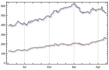
BlurShadow[
   DateListPlot[FinancialData["GE", {2000, 1, 1}], 
      Joined -> True, ImageSize -> 400,
      PlotStyle -> Directive[Thickness[.004], Darker@Red], 
      AspectRatio -> 1/3, GridLines -> Automatic], 
   5, 
   {3, 22}
   ]

Answer 5

Here's a way to do things using Filling that is similar to Mike's approach:

data = Table[{x, Sin[x] + RandomReal[]*0.2}, {x, 0, 2 Pi, Pi/50}];
{xMax, xMin} = {Max@data[[All, 1]], Min@data[[All, 1]]};
{yMax, yMin} = {Max@data[[All, 2]], Min@data[[All, 2]]};
data2 = Plus[{.01 (xMax - xMin), -0.01 (yMax - yMin)}, #] & /@ data;

ListPlot[{data, data2}, Joined -> True, 
 Filling -> {1 -> {{2}, {Directive[Gray, Opacity[0.5]]}}}, 
 PlotStyle -> {{Thickness[0.01], RGBColor[0.7, 0.2, 0.2]}, None}]

Which produces:

Here is an example that uses the ideas in this gradient plot question. However, they're not perfect, and I'm a little tired to dig in and make it great:

ListPlot[data, Joined -> True, 
 Prolog -> 
  Polygon[Join[data, data2], 
   VertexColors -> 
    Join[Blend[{Black, White}, #] & /@ (data[[All, 2]] - 
        data2[[All, 2]]), ConstantArray[White, Length[data]]]], 
 PlotStyle -> {{Thickness[0.01], RGBColor[0.7, 0.2, 0.2]}, None}]

Answer 6

Using DropShadowing: (introduced 2022, v13.1)

 DateListPlot[
      {FinancialData["GOOG", "Close"
      , {{2023, 5, 1}, {2023, 5, 30}}], 
       FinancialData["AAPL", "Close"
       , {{2023, 5, 1}, {2023, 5, 30}}]}
       , Joined -> True
       ,PlotStyle->DropShadowing[]
       ,GridLines->Automatic
       ]

---