How do I draw a pair of buttocks?

Question

I'm trying to develop a function which 3D plot would have a buttocks like shape.

Several days of searching the web and a dozen my of own attempts to solve the issue have brought nothing but two pitiful formulas below.

They have some resemblance to the shape I want, though not quite.

Could you help me to obtain a proper formula?

Here are those bad solutions I've got myself:

ParametricPlot3D[{Sin[y] Sqrt[1 - (Abs[x] - 1)^2], 
  Cos[y] Sqrt[1 - (Abs[x] - 1)^2], x}, {x, -10, 10}, {y, -3 Pi, 3 Pi},
  AspectRatio -> Automatic]

Mathematica graphics

and the following:

Plot3D[((2 Sqrt[30 - x^2 - 2^-x]/3) + Sqrt[1 - (Abs[y] - 1)^2])/2,
   {x, -7, 7}, {y, -7, 7}, AspectRatio -> Automatic]

Mathematica graphics

@YvesKlett Damn, I gotta start collecting those comments ... — Sektor, Nov 25 '14 at 10:36
@Sektor and do not get me started on the edit potential for the title. Just one additional letter would make all the hot post difference ;-) — Yves Klett, Nov 25 '14 at 10:50
@YvesKlett be careful, it happened once :P Evidently, we are... — Kuba, Nov 25 '14 at 10:54
I come back after not checking the site overnight, and this is what I wake up to. — DumpsterDoofus, Nov 25 '14 at 14:47
If only ExampleData[{"Geometry3D", "Beethoven"}] was a full-body model, a judicious use of PlotRange would do it. — , Nov 25 '14 at 16:16
The quality of the responses does seem to be a validation of the merits of this question, albeit a posteriori. — Daniel Lichtblau, Nov 25 '14 at 16:34
When I saw this in the network questions list I thought it was an Arqade link — Steve V., Nov 26 '14 at 00:59
But can you shrink it to 140 characters? http://www.wolfram.com/language/tweet-a-program/ — Rikki, Nov 29 '14 at 00:16
Seriously? A bounty? Hasn't this ridiculous question had enough attention already? — Mr.Wizard, Feb 10 '15 at 14:42
@Rikki would it be a 'tweet' or perhaps more accurately a 'toot' ? — PlaysDice, Oct 18 '15 at 15:34

score 556 · Answer 1 · edited Jun 30 '16 at 00:36

I have to confess that I see this as a proper challenge, as I am usually quite creative in finding/combining functions to provide a desired behavior. So I will give it another try.

Mathematica graphics

which is generated using

box[x_, x1_, x2_, a_, b_] := Tanh[a (x - x1)] + Tanh[-b (x - x2)];
ex[z_, z0_, s_] := Exp[-(z - z0)^2/s]

(*and*)

r[z_, x_] := (*body*).4 (1.0 - .4 ex[z, .8, .15] + 
Sin[2 π x]^2 + .6 ex[z, .8, .25] Cos[2 π x]^2 + .3 Cos[2 π x]) 0.5 (1 + Tanh[4 z]) +
(*legs*)
(1 - .2 ex[z, -1.3, .9]) 0.5 (1 + Tanh[-4 z]) (.5 (1 + Sin[2 π x]^2 +
 .3 Cos[2 π x])*((Abs[Sin[2 π x]])^1.3 + .08 (1 + Tanh[4 z])  )  ) +
(*improve butt*)
.13 box[Cos[π x], -.45, .45, 5, 5] box[z, -.5, .2, 4, 2] - 
0.1 box[Cos[π x], -.008, .008, 30, 30] box[z, -.4, .25, 8, 6] - 
.05 Sin[π x]^16 box[z, -.55, -.35, 8, 18]

(*and finally*) 

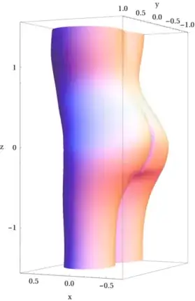
ParametricPlot3D[
(*shift butt belly*)
{.1 Exp[-(z-.8)^2/.6] - .18 Exp[-(z -.1)^2/.4], 0, 0} + {r[z, x] Cos[2 π x], r[z, x] Sin[2 π x],z}, 
{x, 0, 1}, {z, -1.5, 1.5},
PlotPoints -> {150, 50}, Mesh -> None,
AxesLabel -> {"x", "y", "z"}]

Edit What was the strategy in generating the graph (answering the comment of @mcb)

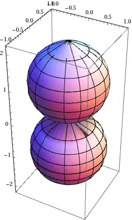
Inspired by some of the solutions here and the fact that the original question seems to head direction Plot3D[] or ParametricPlot3D[], the idea is to use a cylinder as base. I remembered from other work that a parametric curve of type 1+Cos[t] gives something butt-shaped and 1+ a Cos[t] can give something like a torso cross section. To make it a little bit more elliptical I added a 1+Sin[t]^2type. Combining this already goes in the right direction.

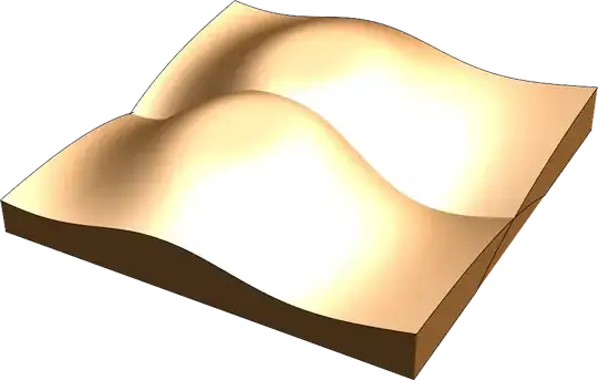
Legs are also not very complicated. Just fold the cylinder into two by,e.g, Abs[Sin[t]]. To make the transition from legs to torso I use a soft step based on Tanh[].

Next step is to push it in and out in the correct way (belly and butt), so there is a shift to the cylinder based on Gaussians.

At the end one adds features like waist, etc. using Gaussians or adjustable smooth box-like functions.

Done, overall not too complicated.

...although I have to say that it is a little bit embarrassing that my "reputation" up to now is mainly from this thread. — mikuszefski, Nov 25 '14 at 18:19
This is the first answer on this site that has literally made me go "what the f—" out loud. So congratulations for that. — , Nov 25 '14 at 18:24
Em-bare-assing? No way. Epic, more like! And who says math ain't sexy now? — Yves Klett, Nov 25 '14 at 19:17
@belisarius Since rotation does not work, have you tried a Legender transform? — Daniel Lichtblau, Dec 01 '14 at 20:35

gpap · Answer 2 · 2014-12-01T20:13:28.487

244

This might get me suspended from the site butt I cannot resist.

The shape you are looking for can probably be approximated (depending how anal you want to be about the outcome) by two assymetric probability distributions. The obvious choices would be a Poasson or a log normal distribution. I will use the latter as it is continuous. Now the bummer is that you have to smoothen them out somehow so I will use an exponential to do that. Since it is the overlap of the two functions that I am interested, I need to add some filling so that the individual sheets don't show (cheeky, I know). I chose Filling->Bottom for that. The final result is shown below (please don't be harse in judging it):

Plot3D[{
  -PDF[LogNormalDistribution[1, 1], (y + .3)^2 + x^2] E^(.8 (y + .7)^2), 
  -PDF[LogNormalDistribution[1, 1], (y - .3)^2 + x^2] E^(.8 (y - .7)^2)
 }, 
 {x, -1.,1.4}, {y, -.9, .9},
 Filling -> Bottom,
 FillingStyle -> Opacity[1],
 PlotStyle -> {Brown, Brown},
 Lighting -> "Neutral",
 Boxed -> False,
 Axes -> False,
 Mesh -> None,
 PlotRange -> {Automatic, Automatic, {-.4, .3}}]

Rendered image of the parametric butt

Cracking!

edited Dec 01 '14 at 20:13

answered Nov 25 '14 at 11:41

gpap

9,707
3
24
66

9

http://youtu.be/FtmjgeEL-tk – Yves Klett Nov 25 '14 at 12:00
It was your comment that started it all :) – gpap Nov 25 '14 at 12:01
11

And good use of misspelling (I think life was better before the advent of the spell checker anyway). – Daniel Lichtblau Nov 25 '14 at 16:26
1

The filling really gives it this little extra! – mikuszefski Nov 25 '14 at 18:14
17

@DanielLichtblau I think you mean spell cheecker. – cubecubed Nov 25 '14 at 22:17
13

@Cammy_the_block Yes, my mistake. Spanks for catching it. – Daniel Lichtblau Nov 25 '14 at 23:49
Filling -> Bottom is fine, but I would use Lighting -> "Subtle" instead of "Neutral"... Mesh would be helpful too, I don't know why you omitted it... – Adrian Nov 26 '14 at 14:08
@gpap; who would have thought... – Eelvex Nov 27 '14 at 02:01
14

"Filling -> Bottom"? Really? – dwa Nov 27 '14 at 08:06
1

@dwa no pun intended... – gpap Nov 27 '14 at 09:49
4

An unusual application of the Lognormal distributtion – wolfies Nov 27 '14 at 15:39
It's "Poisson" not "Poasson" (although the pronunciation is more like the latter) - and I can't fix that damned typo, because "edits must be at least 6 characters long". – peterph Nov 28 '14 at 10:27
Oh, ok. No pun intended right? – peterph Nov 28 '14 at 10:41
@peterps So difficult? :) In addition to your typo correction, use just one synonym elsewhere in your post (e. g. change 'propose' into 'suggest') and voila, you've met the editing requirements. – Nov 28 '14 at 17:03
1

@DanDascalescu why did you edit out the Poasson pun? If feel the original version was so, well, original that just about no editing will be beneficial. – Yves Klett Dec 01 '14 at 11:51
@Yves: it was a pun? As peterph mentioned it was a typo. Plus, I added another pun. – Dan Dascalescu Dec 01 '14 at 12:53
1

@DanDascalescu I´d guess it was intentional by gpap - at least there is no statement here to the opposite. And adding another bottom just does not appeal to me in the sense that the post was so ingeniously authored to begin with that embellishing would do no good. – Yves Klett Dec 01 '14 at 12:57
@YvesKlett: feel free to undo my edit. I won't object. – Dan Dascalescu Dec 01 '14 at 12:58
@DanDascalescu I´d rather leave it to the author - he should have some authority here ;-) – Yves Klett Dec 01 '14 at 12:59
1

@DanDascalescu (@YvesKlett: thanks for the kind words!) I noticed the edit, I just didn't want to re-edit as it would bounce the post and I think the moderators got into a bit of a pickle with all the spam associated with this. But, yep, Poasson was deliberate :) changed it back... – gpap Dec 01 '14 at 20:11
Ass I said: Sassy, that post wass ;-) – Yves Klett Dec 01 '14 at 20:24
@gpap: I'm not a native speaker. Can you explain the Poasson pun? – Dan Dascalescu Dec 02 '14 at 00:27
2

@DanDascalescu Ehm, poasson? – gpap Dec 02 '14 at 16:34

score 132 · Answer 3 · answered Nov 25 '14 at 13:55

132

Parametric Buttocks Manipulator

Manipulate[
 ParametricPlot3D[{
   (e u^p + (1 + (c - a u) (u - 1)) Cos[t]^2) Sin[t],
   (e u^p + (1 + (d - b u) (u - 1)) Cos[t]^2) Cos[t],
   2 u}, {t, -0.2, Pi + 0.2}, {u, 0, 1.1}, Lighting -> "Neutral", Mesh -> None, 
  PlotStyle -> Directive[Specularity[0], RGBColor[0.92, 0.85, 0.73]], Axes -> False],
 {{a, 7}, 2, 10},
 {{b, 2.5}, 1, 3},
 {{c, -0.5}, -1, 0},
 {{d, -0.5}, -1, 0},
 {{e, 0.7}, 0.5, 1},
 {{p, 2.5}, 1, 5}]

enter image description here

answered Nov 25 '14 at 13:55

Simon Woods

84,945
8
175
324

12

It's all about the bass, 'bout the bass, no treble... – rm -rf Nov 25 '14 at 13:58
4

I can't believe I actually spent time to "improve" my answer after seeing yours. This has great silliness potential.. – gpap Nov 25 '14 at 14:05
6

IMO the butt looks nicer with these parameters: http://i.imgur.com/DmFYQTY.png – Öskå Nov 25 '14 at 14:06
22

@Öskå, I agree, your butt is nicer than mine. – Simon Woods Nov 25 '14 at 14:17
1

@gpap ´s not silly. ´s really badass! – Yves Klett Nov 25 '14 at 15:22
10

This only looks like a bra. – Ludwik Nov 25 '14 at 20:01
16

@Ludwik, dammit I knew I should have paid attention in anatomy class! – Simon Woods Nov 25 '14 at 20:33
14

However, the last few lines of code are actually quite buttock-shaped. Was that intentional? – itsbruce Nov 26 '14 at 18:43
the answer above and this answer can be used to make a great creation. I maths is awesome. – Ilaya Raja S May 22 '15 at 05:31

Sjoerd C. de Vries · Answer 4 · 2015-10-18T19:08:25.653

70

Scientific progress! In v10.3 with all the goodies in AnatomyData we can now use the simple code:

Entity["AnatomicalStructure", "Skin"]["Graphics3D"]

Mathematica graphics

Zoom in on the appropriate part and you're done.

pelvisLoc = AnatomyData[Entity["AnatomicalStructure", "Pelvis"], "RegionBounds"]; 
Show[
   Entity["AnatomicalStructure", "Skin"]["Graphics3D"], 
   PlotRange -> pelvisLoc, 
   PlotRangePadding -> {33, 33, 19},
   ViewPoint -> {0.961, 1.62, 0.203}, 
   ViewVertical -> {0.109, 0.284, 1.202}
]

Mathematica graphics

Although not parametric, I thought it would be a nice addition to the other answers.

For those at work: I would advise to leave the Viewpoint where it is.

edited Oct 18 '15 at 19:08

answered Oct 18 '15 at 13:43

Sjoerd C. de Vries

65,815
14
188
323

19

It's a new kind of buttocks, you know. – kirma Oct 18 '15 at 14:22
16

@kirma At least they didn't use you-know-who to stand model here. – Sjoerd C. de Vries Oct 18 '15 at 14:44
6

pelvisLoc is the best function name ever! – gpap Oct 19 '15 at 19:31
Oh yeah! Good ol' C-x M-c M-butterfly – quetzalcoatl Jan 05 '23 at 20:35

score 36 · Answer 5 · edited Nov 25 '14 at 11:54

36

Well, an unusual question to answer, what about something like this

Plot3D[.7*(1 + Tanh[1 - (2*Y^2 + X^2 + X^4)]) - .3*Exp[-X^2/.0025]*
   Exp[-(Y - .1)^2/.15] - .2*(Exp[-(X - .7)^2/.02]*Exp[-(Y - .0)^2/.08] + 
     Exp[-(X + .7)^2/.02]*Exp[-(Y - .0)^2/.08]), {X, -1, 1}, {Y, -1, 1}]

Mathematica graphics

edited Nov 25 '14 at 11:54

Öskå

8,587
4
30
49

answered Nov 25 '14 at 11:42

mikuszefski

4,877
1
14
18

16

Right! You finally put Tanh to some astounding use (I was always wondering what it was good for)! – Yves Klett Nov 25 '14 at 15:20
1

One of my favorites! – mikuszefski Nov 25 '14 at 18:12
20

If I had to guess which body part this represents, my first answer would not be a butt. – Nikolaj-K Nov 27 '14 at 13:42

score 19 · Answer 6 · answered Nov 27 '14 at 15:27

19

Just a combination of Graphics3D objects

Graphics3D[{Scale[
Cylinder[{{0, 0.9, -0.5}, {2, 0.7, 0.5}}, 0.75], {1, 0.95, 1}],  
Scale[Cylinder[{{0, -0.9, 0}, {2, -0.7, 0}}, 0.75], {1.0, 0.95, 1}],
Scale[Cylinder[{{-1.1, 0, 0}, {-0.3, 0, 0}}, 1.5], {1, 1, 0.5}],
Scale[Sphere[{0., 0.75, -0.25}, 1.05], {1.1, 0.9, 1}],
Scale[Sphere[{0., -0.75, 0.1}, 1.05], {1.1, 0.9, 1}],
Sphere[{-0.2, 0, 0.2}, 0.65],
Scale[Sphere[{-0.4, 0, -0.2}, 1.2], {0.6, 1.3, 0.75}],
}, PlotRange -> All, Boxed -> False, 
Lighting -> ({"Spot", ColorData["SouthwestColors"][RandomReal[]], 
   Scaled[#], {Pi/4, 100}} &) /@ RandomReal[{-4, 4}, {5, 3}]]

enter image description here

answered Nov 27 '14 at 15:27

yarchik

18,202
2
28
66

Interesting ansatz...good one. – mikuszefski Nov 27 '14 at 16:02
70

Those hemorrhoids though... – Frigo Nov 30 '14 at 18:34
Well, I guess it is inspired by Fernando Botero sculptures. – mikuszefski Nov 30 '14 at 20:48

How do I draw a pair of buttocks?

6 Answers6

Parametric Buttocks Manipulator

Linked