I'd like to display field lines for a point charge in 3 dimensions

Question

I'd like to display field lines for a point charge in 3 dimensions. Not a force field (short arrows) but continuous field lines that start on the charge.

Answer 1

This is something I have used for my classes. Over time, I've tried to make it more and more user friendly, but that's also made it a little longish. I'll post the complete set of functions, with apologies if it's a bit unwieldy...

As you'll see, I found it does indeed work better in my use cases if I normalize the field, so that we advance along the field lines in more balanced steps. The hardest part in applying these functions is to choose the appropriate seed points.

fieldSolve::usage = 
  "fieldSolve[f,x,x0,\!\(\*SubscriptBox[\(t\), \(max\)]\)] \
symbolically takes a vector field f with respect to the vector \
variable x, and then finds a vector curve r[t] starting at the point \
x0 satisfying the equation dr/dt=\[Alpha] f[r[t]] for \
t=0...\!\(\*SubscriptBox[\(t\), \(max\)]\). Here \[Alpha]=1/|f[r[t]]| \
for normalization. To get verbose output add debug=True to the \
parameter list.";

fieldSolve[field_, varlist_, xi0_, tmax_, debug_: False] := Module[
  {xiVec, equationSet, t},
  If[Length[varlist] != Length[xi0], 
   Print["Number of variables must equal number of initial conditions\
\nUSAGE:\n" <> fieldSolve::usage]; Abort[]];
  xiVec = Through[varlist[t]];
  (* Below, Simplify[equationSet] would cost extra time 
    and doesn't help with the numerical solution, so   don't try to simplify. *)

  equationSet = Join[
    Thread[
     Map[D[#, t] &, xiVec] == 
      Normalize[field /. Thread[varlist -> xiVec]]
     ],
    Thread[
     (xiVec /. t -> 0) == xi0
     ]
    ];
  If[debug, 
   Print[Row[{"Numerically solving the system of equations\n\n", 
      TraditionalForm[(Simplify[equationSet] /. t -> "t") // 
        TableForm]}]]];
  (* This is where the differential equation is solved. 
  The Quiet[] command suppresses warning messages because numerical precision isn't crucial for our plotting purposes: *)

  Map[Head, First[xiVec /.
     Quiet[NDSolve[
       equationSet,
       xiVec,
       {t, 0, tmax}
       ]]], 2]
  ]   

fieldLinePlot[field_, varList_, seedList_, opts : OptionsPattern[]] :=
   Module[{sols, localVars, var, localField, plotOptions, 
    tubeFunction, tubePlotStyle, postProcess = {}}, 
   plotOptions = FilterRules[{opts}, Options[ParametricPlot3D]];
   tubeFunction = OptionValue["TubeFunction"];
   If[tubeFunction =!= None,
    tubePlotStyle = Cases[OptionValue[PlotStyle], Except[_Tube]];
    plotOptions = 
     FilterRules[plotOptions, 
      Except[{PlotStyle, ColorFunction, ColorFunctionScaling}]];
    postProcess = 
     Line[x_] :> 
      Join[tubePlotStyle, {CapForm["Butt"], 
        Tube[x, tubeFunction @@@ x]}]
    ];
   If[Length[seedList[[1, 1]]] != Length[varList], 
    Print["Number of variables must equal number of initial \
conditions\nUSAGE:\n" <> fieldLinePlot::usage]; Abort[]];
   localVars = Array[var, Length[varList]];
   localField = 
    ReleaseHold[
     Hold[field] /. 
      Thread[Map[HoldPattern, Unevaluated[varList]] -> localVars]];
   (*Assume that each element of seedList specifies a point AND the \
length of the field line:*)Show[
    ParallelTable[
     ParametricPlot3D[
         Evaluate[
          Through[#[t]]], {t, #[[1, 1, 1, 1]], #[[1, 1, 1, 2]]}, 
         Evaluate@Apply[Sequence, plotOptions]
         ] &[fieldSolve[
        localField, localVars, seedList[[i, 1]], seedList[[i, 2]]
        ]
       ] /. postProcess, {i, Length[seedList]}
     ]
    ]
   ];

Options[fieldLinePlot] = 
  Append[Options[ParametricPlot3D], "TubeFunction" -> None];

SyntaxInformation[fieldLinePlot] = {"LocalVariables" -> {"Solve", {2, 2}}, 
   "ArgumentsPattern" -> {_, _, _, OptionsPattern[]}};

SetAttributes[fieldSolve, HoldAll];

The main function is fieldLinePlot, but I split it into two functions to be more modular. Also, the problem of where to start drawing the field lines is treated separately because it depends a lot on the particular application.

fieldSolve[f,x,x0,Subscript[t, max]] symbolically takes a vector field f with respect to the vector variable x, and then finds a vector curve r[t] starting at the point x0 satisfying the equation dr/dt = α f[r[t]] for t=0...tmax. Here α = 1/|f[r[t]]| for normalization. To get verbose output add debug=True to the parameter list.

fieldLinePlot[field,varlist,seedList] plots 3D field lines of a vector field (first argument) that depends on the symbolic variables in varlist. The starting points for these variables are provided in seedList.

Each element of seedList={{p1, T1},{p2, T2}...} is a tuple where pi is the starting point of the $i^\mathrm{th}$ field line and Ti is the length of that field line in both directions from Pi.

Here are some examples:

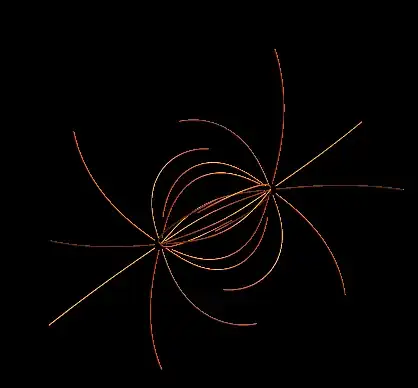
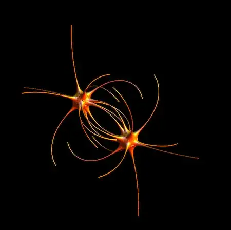
1) Coulomb field of two opposite charges at $\vec{r} = \vec{0}$ and $\vec{r} = (1, 1, 1)$:

Look at the form of seedList to see how the field line starting points and lengths are specified.

seedList = 
  With[{vertices = .1 N[PolyhedronData["Icosahedron"][[1, 1]]]}, 
   Join[Map[{#, 2} &, vertices], 
    Map[{# + {1, 1, 1}, -2} &, vertices]]];

Show[fieldLinePlot[{x, y, z}/
    Norm[{x, y, z}]^3 - ({x, y, z} - {1, 1, 1})/
    Norm[{x, y, z} - {1, 1, 1}]^3, {x, y, z}, seedList, 
  PlotStyle -> {Orange, Specularity[White, 16], Tube[.01]}, 
  PlotRange -> All, Boxed -> False, Axes -> None], 
 Background -> Black]

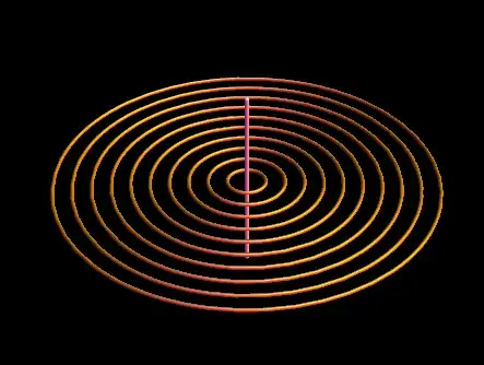
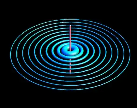
2) Magnetic field of an infinite straight wire:

With[{seedList = Table[{{x, 0, 0}, 6.5}, {x, .1, 1, .1}]
  },
 Show[fieldLinePlot[{-y, x, 0}/(x^2 + y^2), {x, y, z}, 
   seedList, PlotStyle -> {Orange, Specularity[White, 16], Tube[.01]},
    PlotRange -> All, Boxed -> False, Axes -> None], 
  Graphics3D@Tube[{{0, 0, -.5}, {0, 0, .5}}], Background -> Black]]

---

Edit: added variable line thickness to represent field strength

The field lines can be given a color that scales with the field strength (the norm of the vector field along the lines), by specifying a ColorFunction in fieldLinePlot. For example, if the vector field has been defined as a function f2 of variables x,y,z, then you could add the option ColorFunctionScaling -> False, ColorFunction -> Function[{x,y,z,u}, Quiet@Hue[Clip[ Norm[f2[x,y,z]],{0,20}]/20]] as I mention in the comment section.

In this new edit, I added the ability to encode the field strength in the thickness of the field lines instead. This required adding a new option "TubeFunction" which works similarly to ColorFunction. It is a function of the three coordinates x,y,z and returns the radius of the tube representing the field line at that point. To calculate this radius in the examples below, I take the (unscaled) value of the field and get its Norm. Then I scale and constrain it to a reasonable range so that the thickness variations of the field lines don't look too grotesque:

3) Same Coulomb field as above, but with varying field line thickness

f2[x_, y_,z_] := {x, y, z}/Norm[{x, y, z}]^3 - ({x, y, z} - {1, 1, 1})/
   Norm[{x, y, z} - {1, 1, 1}]^3

seedList = 
  With[{vertices = .1 N[PolyhedronData["Icosahedron"][[1, 1]]]}, 
   Join[Map[{#, 2} &, vertices], 
    Map[{# + {1, 1, 1}, -2} &, vertices]]];

fieldLinePlot[f2[x, y, z], {x, y, z}, seedList, 
 PlotStyle -> {Orange, Specularity[White, 16]}, PlotRange -> All, 
 Boxed -> False, Axes -> None, 
 "TubeFunction" -> 
  Function[{x, y, z}, Quiet[Clip[Norm[f2[x, y, z]], {2, 40}]/200]], 
 Background -> Black]

4) Same magnetic field as above, this time with varying line thickness

f3[x_, y_, z_] := {-y, x, 0}/(x^2 + y^2)

With[{seedList = Table[{{x, 0, 0}, 6.5}, {x, .1, 1, .1}]}, 
 Show[fieldLinePlot[f3[x, y, z], {x, y, z}, seedList, 
   PlotStyle -> {Cyan, Specularity[White, 16]}, PlotRange -> All, 
   Boxed -> False, Axes -> None, 
   "TubeFunction" -> 
    Function[{x, y, z}, Quiet[Clip[Norm[f3[x, y, z]], {1, 40}]/200]]],
   Graphics3D@Tube[{{0, 0, -.5}, {0, 0, .5}}], Background -> Black]]

Answer 2

Assuming that the motion of the particle is governed by some force field, you could use NDSolve together with ParametricPlot3D to plot the individual field lines. For example, consider the force field

force[p_] := ({1, 1, 1} - p)/Norm[{1, 1, 1} - p]^3 - p/Norm[p]^3

The equations of motion are given by

p[t_] := {p1[t], p2[t], p3[t]}
eqs := Thread[p''[t] == force[p[t]]]

We also need some initial conditions, for example

ic := {Thread[p[0] == {1, 0, 0}], Thread[p'[0] == {0, 1, 0}]}

The system can then be solved according to

sol = NDSolve[{eqs, ic}, {p1, p2, p3}, {t, 0, 20}]

And the plot of this solution looks like

ParametricPlot3D[p[t] /. sol, {t, 0, 20}]

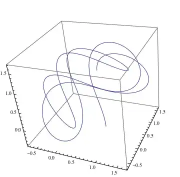
If you want several field lines, you would need to rerun NDSolve for a list of initial conditions.

Edit

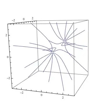
As rcollyer pointed out, this doesn't actually plot the field lines. For that you would need to solve p'[t] == force[p[t]]/Norm[force[p[t]] for which you can still use the method above, e.g.

eq := Thread[p'[t] == -force[p[t]]/Sqrt[force[p[t]].force[p[t]]]]
(* seeds for field lines *)
seeds = Flatten[{0.1 #, 0.1 # + {1, 1, 1}} & /@ 
   N[PolyhedronData["Icosahedron"][[1, 1]]], 1];
sol = NDSolve[{eq, Thread[p[0] == #]}, {p1, p2, p3}, {t, 0, 40}][[1]] & /@ seeds;

ParametricPlot3D[p[s] /. sol, {s, 0, 20}, 
   PlotRange -> {{-3, 3}, {-3, 3}, {-3, 3}}]

Answer 3

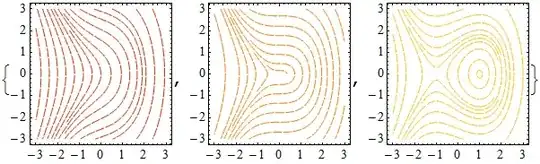
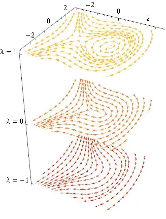
The closest thing in the help files that I can see is this example. It might be of some use.

stackPlots[plots2D : {__Graphics},
  dh_, o : OptionsPattern[Graphics3D]] := Graphics3D[
  MapIndexed[
   Function[{g, index}, g[[1]] /. Arrow[v2d_] :> Arrow[v2d /.
        {x_?NumericQ, y_?NumericQ} :> {x, y, dh index[[1]]}]], 
   plots2D], o]

plotSpacing = 5;

values = {-1, 0, 1};
plots = MapIndexed[
  Function[{\[Lambda], i}, 
   StreamPlot[{y, \[Lambda] - x^2}, {x, -3, 3}, {y, -3, 3}, 
    StreamPoints -> 16, StreamScale -> 0.07,
    StreamStyle -> ColorData["SolarColors"][0.3 i[[1]]]]], values]

stackPlots[plots, plotSpacing, Axes -> True, Boxed -> False, 
 Ticks -> {Automatic, Automatic,
   MapIndexed[{plotSpacing #2[[1]], Row[{"\[Lambda] = ", #1}]} &, 
    values]}]