recreating nyquist regions using FFT python

Question

using python I have sampled a signal and made FFT to see the spectral picture of the time domain signal. the plot bellow shows only 1st and 2nd nyquist zone. I want to expend the spectral image and see the 3rd and 4th nyquist zones.

i have tried to double number of samples but it only expand the previos image two times. where did i go wrong recreating addional nyquist zones? Thanks.

Fs=200e3;#Hz
Ts=1/Fs;
dt=np.arange(0,1,Ts)
f1=10e3;
f2=20e3;
f3=30e3;
y=5*np.sin(2*pi*f1*dt)+5*np.sin(2*pi*f2*dt)+10*np.sin(2*pi*f3*dt)
L=np.size(y)
freq_vec=Fs*np.arange(0,1,Ts)
X=fft(y,L)
plt.plot(freq_vec,abs(X)/(0.5*L))
z=abs(X)

Answer 1

I highly recommend using the DTFT, not the DFT, for this task. The DTFT is defined for all frequencies, unlike the DFT (*).

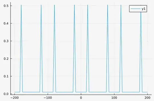
Here's a plot of the magnitude of the DTFT of a sine wave of frequency 20 Hz, sampled at 100 Hz, from -200 to 200 Hz. You can clearly see the different Nyquist zones:

(*) Technically the DFT can be evaluated at any frequency (in other words, for any real $k$). However, the way it is usually implemented in the FFT does not easily allow for this flexibility.

My implementation of the DTFT in Julia. This function returns the DTFT of vector wf evaluated at f0 (in Hz), with sampling frequency fs.

function dtft(wf::Vector{T}, f0, fs = 1.0) where T
    z = -2π*f0/fs
    x = zero(ComplexF64)
    n = 0
    @inbounds @simd for i ∈ eachindex(wf)
        x += wf[i]*cis(z*n)
        n += 1
    end
    x/length(wf)
end