Now that you've selected an answer and I won't be treading on anyone's feet, I can write more freely than before. Whether or not you'll see it is another matter.
There's a reason why Andy's equation worked in your case. And although he achieved a correct answer, he didn't set things up so that you can gain a little more insight into what's going on. That didn't set well with me. So I add something here. (Note that some of the plots produced below were generated by the Desmos grapher web site.)
Here's the obvious plot of \$v_{{\small \text{IN}}\left(t\right)}\$, after the (assumed ideal) bridge rectifier, with \$V_\text{pk}=311\:\text{V}\$ and \$f=50\:\text{Hz}\$:
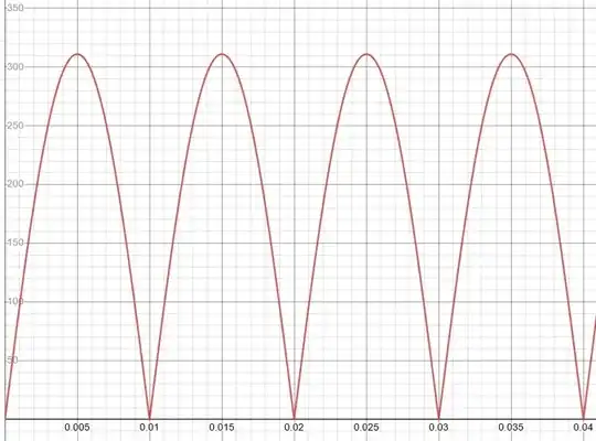
The equation for this is:
$$v_{{\small \text{IN}}\left(t\right)}=V_\text{pk}\cdot\sqrt{\frac12\left[1+\cos\left(4\pi f t+\pi\right)\right]}$$
(If you want to understand why, please read Alfred Centauri's EESE explanation.)
The important issue has to do with inductive charge or Webers (aka: volt-seconds.) The equation should have been written as:
$$W_{\!b}=\int_0^{\frac{1}{2 f}} \left(v_{{\small \text{IN}}\left(t\right)}-v_{{\small \text{C}}\left(t\right)}\right)\:\text{d}t$$
This computes the Webers of charge that will be accumulated into the inductor during one of the half-cycles shown above. Let me explain this equation.
In order to only examine one cycle (which is half the duration of a \$50\:\text{Hz}\$ cycle), I am integrating from \$0\$ to \$\frac12\$ of \$\frac1{f}\$, or \$\frac1{2f}\$. In order to examine the applied volt-seconds here, I need to take the voltage difference between the input source (already described) and the output, which is the capacitor voltage. So a difference is shown there. This voltage difference is then multiplied by the infinitesimal of time and these tiny bits are added up. The units that result from this integration will be volt-seconds or Webers.
Assuming for now that the capacitor voltage is zero (and stays that way for the entire half-cycle -- which isn't true but close enough for now), then the accumulation of Webers over the first half-cycle looks like this curve:
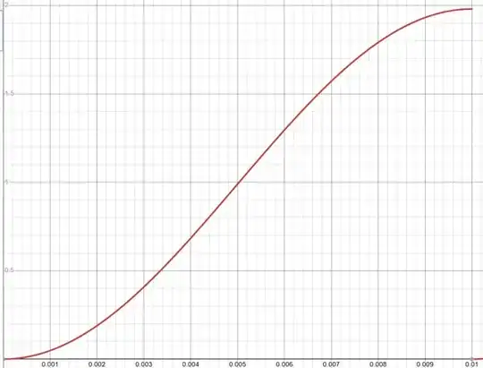
(Computed as \$V_\text{pk}\cdot\frac{1-\mid\sin\left(2\pi f\,t\right)\mid\cdot\cot\left(2\pi f\,t\right)}{2\pi f}\$. Again, with \$V_\text{pk}=311\:\text{V}\$ and \$f=50\:\text{Hz}\$.)
Now, the current in the inductor must at all times be its accumulated Webers, whatever that might be, divided by its inductance. So at the end of the first half-cycle (assuming the capacitor didn't develop a significant voltage), we would expect to see an inductor current of \$\frac{1.98\:\text{Wb}}{131\:\text{mH}}\approx 15.1\:\text{A}\$.
Simulation shows about \$14.0\:\text{A}\$. But simulation also shows that the capacitor voltage had already then risen to about \$40\:\text{V}\$. So we should have docked the \$1.98\:\text{Wb}\$ by \$\frac12\cdot 40\:\text{V}\cdot 10\:\text{ms}=200\:\text{mWb}\$. (Assuming the voltage rise was a nice linear ramp.) Using that better estimate, we'd have computed \$\frac{1.98\:\text{Wb}-200\:\text{mWb}}{131\:\text{mH}}\approx 13.6\:\text{A}\$. That's a little under, now. The reason is that the voltage rise wasn't such a nice linear ramp and instead was always just a little bit underneath such a ramp. So the adjustment was actually too high.
Here's a picture from LTspice simulation of the first half-cycle:
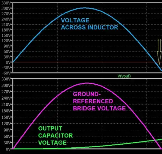
On the bottom pane you can see the input source voltage -- the voltage at the positive side of the bridge rectifier, using the negative side of the bridge rectifier as the ground reference -- as well as the slowly rising capacitor voltage resulting from gradually increasing inductor current due to the building up of Webers in the inductor.
On the top pane you can see the voltage across the inductor. Take note of the yellow arrow which points to the area where the accumulating Webers are negative (before that point they are positive.) This tiny area accounts for the estimate error I just discussed.
The peak current in this first half cycle occurs right at the point just before the Webers being accumulated turn negative. So almost but not quite exactly at the end of the half-cycle.
When the next half-cycle starts, the very first part will start with negative Webers being accumulated, so the inductor current will continue declining slightly before turning back in the positive direction once the input voltage rises over the growing capacitor voltage. More, this time, of the tail end of the half-cycle will also be negative Webers. But again this second half-cycle will have far more positive Webers to accumulate than negative, so the peak current of the inductor will peak still higher during this half-cycle. (Almost twice that from the prior half-cycle.)
As the current in the inductor builds, the capacitor voltage increases more quickly and the balance between accumulated positive and negative Webers shifts. This is where the absolute maximum peak inductor current occurs, declining now as the negative accumulation continues to exceed the positive, before finally settling down to the equilibrium state where there is an exact zero balance between the positive and negative accumulations each half-cycle.
But now the first point here is made: making sense of it through the idea of inductive charge.
With this in hand, I can take you to the same place Andy did, but now using the above physical knowledge to get there. This is an entirely different perspective. Andy used a unitless purely mathematical calculation which provided no insight, but gave the right result almost magically. We are now in a position to find the same result but through a physical understanding.
The concept of steady state is determined by the inductor. It exists when the stored inductive charge in the inductor over the period of one half-cycle neither increases nor decreases, but rather ends at the same value it started at. This is the key concept. If anything other than this occurred, then the inductor would be still charging or discharging and wouldn't be in equilibrium.
The question we now know to ask, and assuming for simplicity the capacitor voltage is also a constant, is,
If we can assume that \$v_{{\small \text{C}}\left(t\right)}\$ can be treated as a constant \$V_{{\small \text{C}}}\$, or that \$v_{{\small \text{C}}\left(t\right)}=V_{{\small \text{C}}}\$, then what's the value of \$V_{{\small \text{C}}}\$ such that:
$$\begin{align*}
\int_0^{\frac{1}{2 f}} \left(v_{{\small \text{IN}}\left(t\right)}-V_{{\small \text{C}}}\right)\:\text{d}t&=0
\\\\
\int_0^{\frac{1}{2 f}} \left(V_\text{pk}\cdot\sqrt{\frac12\left[1+\cos\left(4\pi f t+\pi\right)\right]}-V_{{\small \text{C}}}\right)\:\text{d}t&=0
\\\\
V_\text{pk}\cdot\int_0^{\frac{1}{2 f}} \sqrt{\frac12\left[1+\cos\left(4\pi f t+\pi\right)\right]}\:\text{d}t-V_{{\small \text{C}}}\cdot\int_0^{\frac{1}{2 f}} \text{d}t&=0
\end{align*}$$
The reason this is important is that with a positive capacitor voltage, some of these integrated Webers will be positive and some of them will be negative and, if the value of \$V_{{\small \text{C}}}\$ is just right then these positive and negative values will exactly cancel and the inductor will no longer accumulate Webers from half-cycle to half-cycle.
This is what we mean when we say equilibrium (or perhaps a little more poorly as steady state.) And this is what the output voltage must achieve (assuming a 'large enough' inductor.)
It turns out that the above integration yields the following result:
$$\frac1{f}\left[\frac{V_\text{pk}}{\pi}-\frac{V_{{\small \text{C}}}}{2}\right]=0$$
That will only be zero when \$\frac{V_\text{pk}}{\pi}=\frac{V_{{\small \text{C}}}}{2}\$. Or, put another way, if \$V_{{\small \text{C}}}=\frac{2}{\pi}\cdot V_\text{pk}\$.
What I've done above is true for inductors that are large enough. What this really means is that their ripple current is small enough (because of just how big they are) that their inductive charge doesn't collapse to zero during the half-cycle. (Smaller inductors will run out of inductive charge during the cycle.)
Note this above process is more explanatory, while getting to a similar end. A lesson here is that while short-cuts work (using a mathematical approach stripped of dimensional analysis or understanding of physics), they do not help develop your own skills so as to navigate novel problems you may later face. In essence, they give you a fish rather than teaching you how to fish on your own. My goal here is to teach you fishing so you can think better about new problems ahead.
We've assumed \$V_{{\small \text{C}}}\$ is constant. For large capacitors, this is closer to truth. For smaller capacitors, less so, as their voltage value will vary more during each half-cycle. Regardless, please note that all of the above analysis completely ignored the output capacitance involved! Regardless of the voltage ripple, the above remains true, if a little less simple to analyze. The physics remains. So now we also can see that the capacitor value will affect ripple and that the ripple itself may slightly impact the output voltage. But that when the inductor is large enough, we can closely predict what the average output voltage must be without including the capacitor. You could try reducing the capacitor value by a factor of 1000, for example, and still get similar results out of simulation. (The ripple will be horrible.)
We've learned some things. That's a good thing.
Now, in theory, one should be able to present the input as a source in Laplace form and then apply the Laplace of the following RLC, then perform the inverse Laplace, and all the time-domain stuff would be laid out in front of you.
That's in theory. But practice isn't so neat.
Even in idealized form (eliminating the nearly exponential/logarithmic I/V behavior of the diodes), the input source is \$v_{{\small \text{IN}}\left(t\right)}=V_\text{pk}\cdot\sqrt{\frac12\left[1+\cos\left(4\pi f t+\pi\right)\right]}\$ and that's just not easy (read: 'difficult') to process into the Laplace domain. (If someone can do this for me, I'd be glad to see the result!)
There is still the question about what happens when the inductor is smaller, for example. And it would also be useful to explore how to use knowledge of inductive charge (Webers) both during start-up and also when equilibrium is achieved in order to the consider an inductor's core magnetic cross-section area -- since Webers divided by that area results in Teslas and there are material limitations here. But I'll leave it here, for now.


