I've been trying to solve the following Schrödinger equation numerically, \begin{equation} -(\frac{\partial^2}{\partial y^2} + \frac{\partial^2}{\partial z^2})\Psi + \frac{\sinh^2(y) + \sinh^2(z)}{(\cosh(y) + \cosh(z))^2}\Psi = E\Psi \end{equation}
So far I have written a simple MATLAB code that should solve this, but I keep running into a very weird error. Here's the code:
    clc; clear all;

    N = 30; % Size of the grid. Assume N > 3
    L = 8;  % Size of physical space (L*L)
    h = L/N; % Size of steps

    % Construct d/dx and d/dy matrix which will have size N^2 * N^2
    a = [1; 0; -1; zeros(N - 3,1)];
    A = zeros(N,N);
    for i = 1:N
       A(:, i) = circshift(a, i - 2);
    end
    A(1,N) = 0; A(N, 1) = 0;
    E = eye(N);

    % Do the tensor product
    dx = kron(A, E)./(2*h);
    dy = kron(E, A)./(2*h);

    % Construct the potential matrix
    v = @(x,y) 10*(sinh(x)^2 + sinh(y)^2)/(cosh(x) + cosh(y))^2;
    V = zeros(N*N,N*N);
    for i = 1:N
       for j = 1:N
          pos = j + N*(i - 1);
          V(pos, pos) = v(-L/2 + h*(i-1), -L/2 + h*(j-1));
       end
    end

    % Now construct the Hamiltonian matrix
    H = -dx^2 - dy^2 + V;

    [Psi, D] = eig(H);
    eval = diag(D);

    [useless, perm] = sort(eval);
    eval = eval(perm); Psi = Psi(:,perm);

    %% Plot a choice of Psi
    fprintf('Preparing the plot... \n');
    k = 0;
    PsiFn = zeros(N,N);

    for j = 1:N
        for i = 1:N
            PsiFn(i,j) = Psi(i + N*(j - 1), k + 1);
        end
    end
    [y,z] = meshgrid(-L/2:h:L/2 - h);
    % Ploting |Psi|^2
    figure;
    surf(y,z,PsiFn);
%surf(y,z,abs(PsiFn),'EdgeColor','none','LineStyle','none','FaceLighting','phong');
The idea of the code is really simple. Basically I divide the region I'm trying to solve the equation on into small grids ($N \times N$). Then any function can be written as $N^2$-dimensional vector. For example if my region is $2 \times 2$ then I can represent a function $f$ with values $f(1,1) = 1, f(1,2) = 2, f(2,1) = 3$ and $f(2,2) = 4$ by a vector $\mathbf{f} = (1,2,3,4)$. By doing this I can turn the operator (i.e. the Hamiltonian) \begin{equation} H = -(\frac{\partial^2}{\partial y^2} + \frac{\partial^2}{\partial z^2}) + \frac{\sinh^2(y) + \sinh^2(z)}{(\cosh(y) + \cosh(z))^2} \end{equation} into a matrix. Then the eigenvalues and the solution function (i.e. the energy level and the wavefunction) are given by the eigenvalues and eigenvectors of the operator $H$ which are found from MATLAB eig(...) function. Then I simply rearrange the output from eig(...) so that the first eigenvector corresponding to the one with lowest energy.
Everything seems to make sense but the plot of the output for the solution that meant to corresponding to the ground state looks like
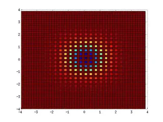
Which is unexpected for an obvious reason. The shape is roughly right but there are gaps between every second columns and rows. I've tried running the same code on a problem with known analytic solution like 2D Quantum Harmonic Oscillator, I still get the same result and the eigenvalues are wrong as well.
So if anyone could point out to me what causes the problem and how could I fix it that would be great.
Alternatively, could anyone tell me a better way to solve this problem. Maybe a sample MATLAB or Mathematica code or just any numerical technique that you think might work better than what I'm currently using.