Conditional expectation $\mathbb E(Y \mid X \in B)$ instead of $\mathbb E(Y \,|\, X = x)$ (generalization of Shorack's PFS Notation 7.4.1)

Question

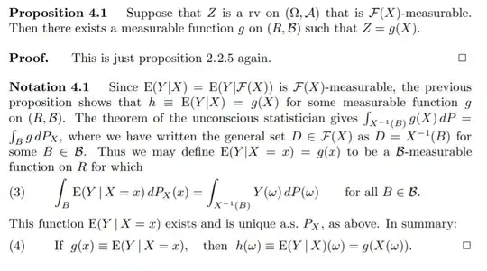
In Shorack's Probability for Statisticians Notation 7.4.1, he notes that the conditional expectation (defined in the measure theoretic way) $\mathbb E(Y\mid X)$ is $g(X)$ for some measurable $g :(\mathbb R, \mathcal B_\mathbb R) \to (\mathbb R, \mathcal B_\mathbb R)$. He then defines $\mathbb E(Y \mid X=x)$ as simply $g(x)$. For conditional probabilities, I'm pretty sure this means that $P(A \mid X=x)$ will be defined as $\mathbb E(1_A \mid X=x)$. I'm not entirely confident that this measure-theoretic definition of conditional probability conditioned on $X=x$ matches with the classical notion of conditional probability, so if someone could shed some light on that too that'd be great.

Here's a picture of the relevant section from the book.

My question is: is there a generalization of this definition to $\mathbb E(Y\mid X\in B)$ for some Borel set $B \in \mathcal B_\mathbb R$?

Looking at this question/answer When do the measure-theoretic and elementary definitions of conditional probability/expectation coincide?, it seems like the generalization would require dividing $P(X\in B)$, which may not be possible since it could be $0$. In that case, why is it that we can have a general definition of $\mathbb E(Y\mid X=x)$ but not of $\mathbb E(Y\mid X\in B)$?

Answer 1

The measure theoretic approach to conditional probability / expectation provides a unifying framework that avoids separate argumentation for "discrete" and "continuous" random variables. One of the first examples/exercises that you will encounter is a verification that the measure theoretic $P(Y|X)$ and $E(Y|X)$ are indeed generalizations of the classical concepts. For example:

Claim: Let $X$ be a discrete random variable taking finitely many values $x_1,\ldots,x_k$, each with positive probability. Then $$E(Y\mid X)= \sum_{i=1}^k \frac{E(Y; X=x_i)}{P(X=x_i)} I(X=x_i).\tag1$$

Formula (1), which follows from the definition of conditional expectation, is an explicit representation of the measure-theoretic $E(Y\mid X)$ as a linear combination of indicators of the events $\{X=x_1\}$, $\ldots$, $\{X=x_k\}$. Another way to write (1) is: $E(Y\mid X) = g(X)$ where the function $g$ is defined by $$g(x)=\begin{cases}\displaystyle\frac{E(Y;X=x_i)}{P(X=x_i)}&\text{if $x=x_i$}\\0&\text{otherwise}\end{cases}.$$ We next remark that if we adopt the notation $$E(Y\mid X=x):=g(x),$$ then this notation coincides with the elementary concept of conditional expectation given $X=x$ for discrete $X$. You can prove that this correspondence holds in the continuous case too; this is the motivation for Notation 4.1 in the passage that you excerpted.

As another exercise, you can prove a measure-theoretic analog of (1) for $P(A\mid X)$, namely $$P(A\mid X)=\sum_{i=1}^k \displaystyle\frac{P(A; X=x_i)}{P(X=x_i)}I(X=x_i).$$ So yes, the notation $P(A\mid X=x_i)$ matches the classical notion.

In the measure-theoretic development the quantity $E(X\mid A)$, for $A$ an event, retains the same meaning as in the elementary approach: it's still $E(X;A)/P(A)$. There's no need to redefine in a "measure-theoretic way", since the numerator and denominator are well defined and their ratio makes sense as long as $P(A)$ is not zero. This is not a limitation, since typically the only events we condition on that have probability zero are those of the form $\{X=x\}$; and we've already given a rigorous interpretation to the notation $E(Y\mid X=x)$. Either that, or our arguments involve conditional expectations in their original form $E(Y\mid X)$ and we avoid conditioning on events at all.

Answer 2

Why not continue the analogy and set $\mathbb{E}(Y \, \mid \, A) = \mathbb{E}(Y , \mid \, 1_{A} = 1)$? In this case, you can check that $\mathbb{E}(Y \, \mid \, 1_{A} = 1) = \frac{\mathbb{E}(Y : A)}{\mathbb{P}(A)}$ so that it is consistent with the naive approach. Further, it's worth noting that $\mathbb{E}(Y \, \mid \, 1_{A})$ has the form \begin{equation*} \mathbb{E}(Y \, \mid \, 1_{A}) = \left\{ \begin{array}{r l} \frac{\mathbb{E}(Y : A)}{\mathbb{P}(A)}, & \text{in} \, \, A, \\ \frac{\mathbb{E}(Y : A^{c})}{\mathbb{P}(A^{c})}, & \text{in} \, \, A^{c}. \end{array} \right. \end{equation*} I leave the confirmation of these identities as exercises, which are not too hard since $\sigma(1_{A}) = \{\phi, A, A^{c}, \Omega\}$.

An interesting fact that's worth mentioning here is that if $Y,X$ are two real random variables (you could also use random vectors, but I won't), if $\mu_{X}$ is the law of $X$, and if $Y$ is integrable, then \begin{equation*} \mathbb{E}(Y \, \mid \, X = x) = \lim_{\epsilon \to 0^{+}} \frac{\mathbb{E}(Y : X \in [x - \epsilon, x + \epsilon])}{\mathbb{P}\{X \in [x- \epsilon, x + \epsilon]\}} \quad \text{for} \, \, \mu_{X}\text{-a.e.} \, \, x \in \mathbb{R} \end{equation*} This follows from the Besicovitch Differentiation Theorem (cf. Chapter 5 of Sets of Finite Perimeter and Geometric Variational Problems by Maggi); I don't know an easier way to prove it in general. Replacing $Y$ by $1_{A}$ for suitable events $A$, we can also use this to compute probabilities conditioned on $\{X = x\}$.

On the topic of "conditioning on sets of measure zero," there is yet another fact worth mentioning. Let $U$ be a bounded open subset of $\mathbb{R}^{d}$ with smooth boundary, fix $x \in U$, and let $B^{x}$ be be a standard Brownian motion with $B^{x}_{0} = x$. Let $\tau_{U}$ be the first time $B^{x}$ reaches $\partial U$. It turns out that there is another process $\tilde{B}^{x}$ such that, for each $t \geq 0$, $B^{x}_{t}$ conditioned on $\{\tau_{U} \geq T\}$ converges in distribution to $\tilde{B}^{x}_{t}$ as $T \to \infty$. That is, \begin{equation*} \mathbb{E}(f(\tilde{B}^{x}_{t})) = \lim_{T \to \infty} \frac{\mathbb{E}(f(B_{t}^{x}) : \tau_{U} \geq T)}{\mathbb{P}(\tau_{U} \geq T)}. \end{equation*} Note that $\tau_{U} < \infty$ almost surely so here, as in the last paragraph, we have "(asymptotically) conditioned on a set of measure zero." I don't know if it's possible to interpret the statement "$\tilde{B}^{x}$ equals $B^{x}$ conditioned on $\tau_{U} = \infty$" in a more rigorous way. (More generally, in the theory of stochastic process, the previous construction is called a Yaglom limit.)