The Constant Elasticity of Variance (CEV) process is a one dimensional diffusion process given by the following stochastic differential equation.
\begin{equation} d X_t = \mu X_t \cdot dt + \sigma X_t^\beta \cdot d B_t \tag{1} \end{equation}
where $\mu,\sigma,\beta$ are positive real parameters and $B_t$ is the Brownian motion. In what follows we assume that the starting value of the process reads $X_0 = x > 0$ and that $\beta > 1 $. The infinitesimal generator of this process reads $ {\mathfrak G}_z := \mu z d/d z + \sigma^2/2 z^{2 \beta} d^2/d z^2$ . The eigen-functions of this operator $ {\mathfrak G}_z \phi^{\pm} (z) = \lambda \phi^{\pm}(z) $ to the eigenvalue $\lambda > 0 $ are given below:
\begin{eqnarray} \phi^{+}(z) &=&U\left(\frac{\lambda}{2(-1+\beta) \mu}, 1+ \frac{1}{2(-1+\beta)}, \frac{\mu z^{2-2\beta} }{(-1+\beta) \sigma^2} \right) \tag{2a} \\ \phi^{-}(z) &=& L_{-\frac{\lambda}{2(-1+\beta) \mu}}^{(\frac{1}{2(-1+\beta)})} \left( \frac{\mu z^{2-2\beta} }{(-1+\beta) \sigma^2}\right) \tag{2b} \end{eqnarray}
where $U$ is the confluent hypergeometric function and $L$ is the generalized Laguerre polynomial. We have checked that $U(z)$ is a strictly increasing function of $z$.
Now, by using the theory of diffusion processes, see section 4.6 pages 128-134 in
Ito, K.; McKean, H. P. jun., Diffusion processes and their sample paths, Berlin-Heidelberg-New York: Springer-Verlag. XVII, 321 p. (1965). ZBL0127.09503.
, we have found the Laplace transform of the first hitting time $\tau_y := inf(s>0:X_s = y)$ of a horizontal barrier $b$ by this process. The quantity in question reads:
\begin{eqnarray} E_x \left[ e^{-\lambda \tau_y} \right] = \frac{\phi^{+}(x)}{\phi^{+}(y)} \quad \mbox{for $x \le y$} \tag{3} \end{eqnarray}
Now, by inverting the Laplace transform in $(3)$, by using the Bromwich integral and then the Cauchy theorem, we have expressed the probability density function of the first hitting time $n_x(t;y) := P_x\left( \tau_y \in dt\right)/dt $ as follows:
\begin{eqnarray} n_x(t;y) = \sum\limits_{p=1}^\infty \underbrace{ \frac{U\left( -\zeta_p^{(y;\mu,\sigma,\beta)}, 1+ \frac{1}{2(-1+\beta)}, \frac{\mu x^{2-2\beta}}{(-1+\beta) \sigma^2} \right)}{ \zeta_p^{(y;\mu,\sigma,\beta)} U^{(1,0,0)}\left( -\zeta_p^{(y;\mu,\sigma,\beta)}, 1+ \frac{1}{2(-1+\beta)}, \frac{\mu y^{2-2\beta}}{(-1+\beta) \sigma^2} \right) } }_{{\mathfrak w}_p^{(y;\mu,\sigma,\beta)}} \cdot \underline{(2 (-1+\beta) \mu \zeta_p^{(y;\mu,\sigma,\beta)} ) \cdot e^{-2 (-1+\beta) \mu \cdot \zeta_p^{(y;\mu,\sigma,\beta)} \cdot t}} \tag{5} \end{eqnarray}
As we can see the quantity in $(5)$ is an infinite linear combination of exponential distributions with weights $ \left( {\mathfrak w}_p^{(y;\mu,\sigma,\beta)} \right)_{p=1}^\infty $ that sum up to unity. Here $ \left( \zeta_p^{(y;\mu,\sigma,\beta)} \right)_{p=1}^\infty $ are zeros of the function $ {\mathbb R}_+ \ni \lambda \rightarrow U(-\lambda,1+ \frac{1}{2(-1+\beta)}, \frac{\mu y^{2-2\beta}}{(-1+\beta) \sigma^2}) \in {\mathbb R} $.
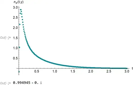
Now we took the following process parameters $\mu,\sigma,\beta = 3/2,1/2,5/2$ and the first value and the barrier $x,y = 3/2, 5/2 $ and we plotted the quantity $(5)$ below. We also verified the normalization numerically. Here we go:
{\[Mu], \[Sigma], \[Beta]} = {3/2, 1/2, 5/2};
(*Here x\[LessEqual]y*)
{x, y} = {3/2, 5/2};
SetOptions[FindRoot, WorkingPrecision -> mprec, PrecisionGoal -> prec];
mzeros = [Lambda] /.
   Table[FindRoot[
     HypergeometricU[-[Lambda],
       1 + 1/(2 (-1 + [Beta])), ([Mu] y^(
        2 - 2 [Beta]))/((-1 + [Beta]) [Sigma]^2)] == 0, {[Lambda],
       n}], {n, 0, 50}];
mzeros = Sort[#[[1]] & /@ Tally[mzeros]];
ts = Array[# &, {300}, {1/100, 3}];
vals = {#,
     Total[Table[
       HypergeometricU[-mzeros[[p]],
         1 + 1/(2 (-1 + [Beta])), ([Mu] x^(
          2 - 2 [Beta]))/((-1 + [Beta]) [Sigma]^2)]/
!(*SuperscriptBox[(HypergeometricU),
TagBox[
RowBox[{"(",
RowBox[{"1", ",", "0", ",", "0"}], ")"}],
Derivative],
MultilineFunction->None])[-mzeros[[p]],
         1 + 1/(2 (-1 + [Beta])), ([Mu] y^(
          2 - 2 [Beta]))/((-1 + [Beta]) [Sigma]^2)] (2 (-1 +

[Beta]) [Mu]) Exp[-2 (-1 + [Beta]) [Mu] mzeros[[p]] #], {p, 1,
        Length[mzeros]}]]} & /@ ts;
ListPlot[vals, PlotRange :> All,
 AxesLabel -> {"t", "!(*SubscriptBox[(n), (x)])(t,y)"}]
f = Interpolation[vals];
NIntegrate[f[xi], {xi, 0.01, 3}]
As you can see the distribution in question has a correct shape and a correct normalization. The negative values close to the origin are due to a numerical error.
Having said all this my question would be how do we evaluate the limit of $\beta \rightarrow 1_+$. In this case the process tends towards the geometric Brownian motion and as such we should have:
\begin{equation} \lim_{\beta \rightarrow 1_+} n_x(t;y) \stackrel{(??)}{=} \frac{\left| \log(\frac{y}{x} )\right|}{\sqrt{2 \pi t^3} \sigma} e^{-\frac{1}{2 \sigma^2 t} \left[ \log(\frac{y}{x} - (\mu - \frac{\sigma^2}{2} ) t\right]^2} \end{equation}
as shown in a previous question on a similar topic.
How do we work out this limit analytically in our framework?
Update:
We have verified numerically that the Laplace transform $ (3) $ approaches the correct limits when $ \beta \rightarrow 1_+ $. See code below:
    {lmb, mu, sig} = RandomReal[{0, 1}, 3, WorkingPrecision -> 50];
    x = RandomReal[{0, 1}, WorkingPrecision -> 50];
    y = RandomReal[{x, 2}, WorkingPrecision -> 50];
    NN = 100;
    HypergeometricU[lmb/mu NN, NN, NN (2 mu/sig^2) x^(-1/NN)]/
     HypergeometricU[lmb/mu NN, NN, NN (2 mu/sig^2) y^(-1/NN)]
    (x/y)^((-2 mu + sig^2 + 2 Sqrt[2 lmb sig^2 + (mu - sig^2/2)^2])/(
      2 sig^2))
0.275584165705622319278498109409236772998453 + 0.*10^-50 I
0.2729011283963510407220223125184479965801097988605
