Obtaining joint distributions and conditional distributions using Mathematica

Question

I have two multivariate Gaussian distributions $p(x)$ and $p(z)$ with mean vectors $m_x$ and $m_z$, and covariance matrices $\Sigma_x$ and $\Sigma_z$. my model is a simple linear model $x = W z+n$ where $n$ is a noise vector with mean $0$ and diagonal covariance matrix of the form $\sigma^2 I$, where $I$ is the identity matrix.

I observe the variable $x$. now how can I calculate the joint distribution $p(x,z)$ and the conditional distributions $p(x|z)$ and $p(z|x)$?

Answer 1

As I use this a lot in my own research, let me answer your question by generalizing it to possibly larger dimensions and with a possibly correlated joint probability.

Let me define the following function

 ConditionalMultinormalDistribution::usage ="ConditionalMultinormalDistribution[pdf,val,idx] 
returns the conditional MultiNormal PDF from the joint PDF pdf while setting the variables 
of index idx to values vals"

so that for example:

m = Table[i, {i, 3}];
S = Table[i + j, {i, 3}, {j, 3}]/20 + DiagonalMatrix[Table[1, {3}]];
pdf = MultinormalDistribution[m, S];
cpdf = ConditionalMultinormalDistribution[pdf, {1, 5}, {1, 3}]

(* NormalDistribution[327/139, 317/278] *)

or slightly less trivially,

m = Table[i, {i, 5}];
S = Table[i + j, {i, 5}, {j, 5}]/20 + DiagonalMatrix[Table[1, {5}]];
pdf = MultinormalDistribution[m, S];
cpdf = ConditionalMultinormalDistribution[pdf, {1, 1, 1}, {1, 3, 5}]

(* MultinormalDistribution[{1, 63/23}, {{35/32, 5/32}, {5/32, 885/736}}] *)

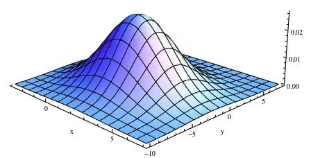
ContourPlot[PDF[cpdf, {x, y}], {x, -2, 4}, {y, 0, 6}, PlotRange -> All,
PlotPoints -> 50, Contours -> 15]

The actual code:

ConditionalMultinormalDistribution[pdf_, val_, idx_] := Module[
    {S = pdf[[2]], m = pdf[[1]], odx, Σa, Σb, Σc, μ2, S2, idx2, val2},
    odx  = Flatten[{Complement[Range[Length[S]], Flatten[{idx}]]}];
    Σa   = (S[[odx]] // Transpose)[[odx]];
    idx2 = Flatten[{idx}];
    val2 = Flatten[{val}];
    Σc   = (S[[odx]] // Transpose)[[idx2]] // Transpose;
    Σb   = (S[[idx2]] // Transpose)[[idx2]];
    μ2   = m[[odx]] + Σc.Inverse[Σb].(val2 - m[[idx]]);
    S2   = Σa - Σc.Inverse[Σb]. Transpose[  Σc];
    S2   = 1/2 (S2 + Transpose[S2]);
    If[
        Length[μ2] == 1, 
        NormalDistribution[μ2 // First, Sqrt[S2 // First // First]], 
        MultinormalDistribution[μ2, S2]
    ]
] /; Head[pdf] == MultinormalDistribution

Update

It might also be of use to have a function which defines a new `MultinormalDistribution distribution from an old one, given some sets of linear equations relating variables together.

ConditionalDistribution::usage = \
"ConditionalDistribution[pdf,vars,equation] returns the 
 set of newvar,substitution rule and pdf corresponding to eliminating \
the first of the variables in the given equation";

     ReturnMarginal::usage = "ReturnMarginal is an option for
  ConditionalDistribution which specifies if the marginal should be \
returned as well; Default Not";

EliminateVariables::usage = "EliminateVariables is an option for
  ConditionalDistribution which specifies which variables 
  should be eliminated; Default is  set of first variables in 
  eqns";

Options[ConditionalDistribution] = {EliminateVariables -> {}, 
   ReturnMarginal -> False};

The actual code is:

  ConditionalDistribution[pdf_, yy_, eqns_, opts : OptionsPattern[]] :=

  Module[{nyy, rs, aa, yyc, npdf, vars, eqns2, tpdf, marg},
  vars = OptionValue[EliminateVariables];
  vars = If[Length[vars] == 0,
    #[[1, 1]] & /@ eqns, vars];
  vars/Print;
  nyy = Select[yy, FreeQ[vars, #] &];
  eqns2 = # == 0 & /@ nyy;
  rs = Solve[eqns, vars][[1]];
  aa = Normal[CoefficientArrays[#, yy]] & /@ Join[eqns, eqns2]; 
  aa = Last /@ aa;
  yyc = Delete[aa.yy /. rs, {#} & /@ Range[Length@vars]];
  npdf = ConditionalMultinormalDistribution[
    tpdf = TransformedDistribution[aa.yy, 
      yy \[Distributed] pdf], #[[2]] & /@ eqns, Range[Length@vars]];
  marg = PDF[
    MarginalDistribution[tpdf, Range[Length@vars]], #[[2]] & /@ 
     eqns];
  If[OptionValue[ReturnMarginal], {yyc \[Distributed] npdf, rs, 
    marg},
   {yyc \[Distributed] npdf, rs}]
  ]

and it works as follows:

   pdf = MultinormalDistribution[Table[0, {5}],Table[Exp[-(i - j)^2], {i, 5}, {j, 5}]];
   {def, rs} = 
   ConditionalDistribution[pdf, 
   var = {Subscript[x, 1], Subscript[x, 2], Subscript[x, 4], 
   Subscript[x, 3], Subscript[x, 5]}, 
   eqn = {Subscript[x, 1] + Subscript[x, 2] == a}] // Simplify

Answer 2

To get the joint density of two distributions, you need to use ProductDistribution. For example, consider the two distributions $p(x)$ and $p(y)$:

px = NormalDistribution[2, 2];
py = NormalDistribution[-2, 3];

(* visualize *)
{Plot[PDF[px, x], {x, -3, 7}, PlotRange -> All],  
 Plot[PDF[py, y], {y, -10, 8}, PlotRange -> All]} // GraphicsRow

Now obtain the joint distribution $p(x,y)$ and visualize:

pxy = ProductDistribution[px, py];
Quiet@Plot3D[PDF[pxy, {x, y}], {x, -3, 7}, {y, -10, 8}, PlotRange -> All, AxesLabel -> {"x", "y"}]

The conditional distribution $p(x|y)$ is then simply the ratio of the joint distribution to the marginal of $y$.

pcxy = PDF[pxy, {x, y}]/PDF[MarginalDistribution[pxy, 2], x]
Quiet@Plot3D[pcxy, {x, -3, 12}, {y, -10, 8}, PlotRange -> All, AxesLabel -> {"x", "y"}]