How to solve coupled multi-variable polynomials?

Question

The following code generates two polynomials $q_1$ and $q_2$ in complex variables p and c:

pp[n_] := If[n > 0, pp[n - 1]^2 + c, p];
q1 = PolynomialQuotient[pp[4] - p, pp[2] - p, p];
q2 = PolynomialRemainder[D[pp[4], p] - 1, q1, p];

I would like to eliminate p and generate either a single polynomial in c or complex numerical solutions to c. Eliminate[] works for similar problems of lower order but never returns a result for this one.

Eliminate[{q1 == 0, q2 == 0}, p]

(* no result returned *)

If I get a solution to that problem, the next thing I need to do is generalize the "1" in the $q_2$ line to a variable t, so I can calculate c[t] where Abs[t]==1.

q2 = PolynomialRemainder[D[pp[4, c], p] - t, q1, p];

Thanks in advance for any help.

UPDATE: In the course of trying proposed solutions to this, I came upon what appears to be a bug, discussed HERE

Answer 1

Part 1 - Eliminate p

I am not sure this is what you are looking for but both Solve and Reduce give solutions.

When I evaluate q1 and q2 I get

pp[n_Integer] := If[n > 0, pp[n - 1]^2 + c, p]

q1 = PolynomialQuotient[pp[4] - p, pp[2] - p, p]
(* 1 + 2 c^2 + 3 c^3 + 3 c^4 + 
 3 c^5 + c^6 + (2 c + c^2 + 2 c^3 + c^4) p + (c + 5 c^2 + 6 c^3 + 
    12 c^4 + 6 c^5) p^2 + (1 + 4 c^2 + 4 c^3) p^3 + (4 c + 3 c^2 + 
    18 c^3 + 15 c^4) p^4 + (2 c + 6 c^2) p^5 + (1 + 12 c^2 + 
    20 c^3) p^6 + 4 c p^7 + (3 c + 15 c^2) p^8 + p^9 + 6 c p^10 + p^12 *)

q2 = PolynomialRemainder[D[pp[4], p] - 1, q1, p]
(* 15 + 32 c^2 + 48 c^3 + 48 c^4 + 48 c^5 + 
 16 c^6 + (16 c + 16 c^2 + 16 c^3) p + (16 c + 48 c^2 + 80 c^3 + 
    160 c^4 + 80 c^5) p^2 + 
 32 c^2 p^3 + (16 c + 32 c^2 + 192 c^3 + 160 c^4) p^4 + 
 16 c p^5 + (96 c^2 + 160 c^3) p^6 + (16 c + 80 c^2) p^8 + 16 c p^10 *)

Now apply Solve

solution = 
 Solve[{1 + 2 c^2 + 3 c^3 + 3 c^4 + 3 c^5 + 
     c^6 + (2 c + c^2 + 2 c^3 + c^4) p + (c + 5 c^2 + 6 c^3 + 
        12 c^4 + 6 c^5) p^2 + (1 + 4 c^2 + 4 c^3) p^3 + (4 c + 
        3 c^2 + 18 c^3 + 15 c^4) p^4 + (2 c + 6 c^2) p^5 + (1 + 
        12 c^2 + 20 c^3) p^6 + 4 c p^7 + (3 c + 15 c^2) p^8 + p^9 + 
     6 c p^10 + p^12 == 0,
   15 + 32 c^2 + 48 c^3 + 48 c^4 + 48 c^5 + 
     16 c^6 + (16 c + 16 c^2 + 16 c^3) p + (16 c + 48 c^2 + 80 c^3 + 
        160 c^4 + 80 c^5) p^2 + 
     32 c^2 p^3 + (16 c + 32 c^2 + 192 c^3 + 160 c^4) p^4 + 
     16 c p^5 + (96 c^2 + 160 c^3) p^6 + (16 c + 80 c^2) p^8 + 
     16 c p^10 == 0}, {c, p}, Complexes];

There is a long list of solutions (some of which have Root) but I won't use up the space showing them. Here is the first:

solution[[1]]
(* {c -> 1/4 - I/2, p -> -(I/2)} *)

Part 2 - Introduce variable t

q2 is changed to include a variable t in place of the 1.

q2 = PolynomialRemainder[D[pp[4], p] - t, q1, p]
(* 16 + 32 c^2 + 48 c^3 + 48 c^4 + 48 c^5 + 
 16 c^6 + (16 c + 16 c^2 + 16 c^3) p + (16 c + 48 c^2 + 80 c^3 + 
    160 c^4 + 80 c^5) p^2 + 
 32 c^2 p^3 + (16 c + 32 c^2 + 192 c^3 + 160 c^4) p^4 + 
 16 c p^5 + (96 c^2 + 160 c^3) p^6 + (16 c + 80 c^2) p^8 + 16 c p^10 -
  t *)

The expression handed to Solve is modified accordingly

solT = Solve[{1 + 2 c^2 + 3 c^3 + 3 c^4 + 3 c^5 + 
      c^6 + (2 c + c^2 + 2 c^3 + c^4) p + (c + 5 c^2 + 6 c^3 + 
         12 c^4 + 6 c^5) p^2 + (1 + 4 c^2 + 4 c^3) p^3 + (4 c + 
         3 c^2 + 18 c^3 + 15 c^4) p^4 + (2 c + 6 c^2) p^5 + (1 + 
         12 c^2 + 20 c^3) p^6 + 4 c p^7 + (3 c + 15 c^2) p^8 + p^9 + 
      6 c p^10 + p^12 == 0, 
    16 + 32 c^2 + 48 c^3 + 48 c^4 + 48 c^5 + 
      16 c^6 + (16 c + 16 c^2 + 16 c^3) p + (16 c + 48 c^2 + 80 c^3 + 
         160 c^4 + 80 c^5) p^2 + 
      32 c^2 p^3 + (16 c + 32 c^2 + 192 c^3 + 160 c^4) p^4 + 
      16 c p^5 + (96 c^2 + 160 c^3) p^6 + (16 c + 80 c^2) p^8 + 
      16 c p^10 == t}, {c, p}, Complexes];

Again there are many solutions.

I don't believe there is any hope to create a functionc[t] for that can be used as an input to Plot.

The first solution was used to form a table of values that could be input to ListPlot.

First a table of complex numbers whose absolute value is unity is formed.

tList = Table[k + I Sqrt[1 - k^2], {k, -1, 1, 0.1}]
(* {-1. + 0. I, -0.9 + 0.43589 I, -0.8 + 0.6 I, -0.7 + 
  0.714143 I, -0.6 + 0.8 I, -0.5 + 0.866025 I, -0.4 + 
  0.916515 I, -0.3 + 0.953939 I, -0.2 + 0.979796 I, -0.1 + 0.994987 I,
  0. + 1. I, 0.1 + 0.994987 I, 0.2 + 0.979796 I, 0.3 + 0.953939 I, 
 0.4 + 0.916515 I, 0.5 + 0.866025 I, 0.6 + 0.8 I, 0.7 + 0.714143 I, 
 0.8 + 0.6 I, 0.9 + 0.43589 I, 1. + 0. I} *)

This is used as the input t to get a table of c[t].

solT1 = Table[{t, N[solT[[1, 1, 2]], 30]}, {t, tList}]
(* {{-1. + 0. I, -1.93971 + 0. I}, {-0.9 + 
   0.43589 I, -1.94168 + 0.000929621 I}, {-0.8 + 0.6 I, -1.94071 - 
   0.0000163376 I}, {-0.7 + 0.714143 I, -1.94177 + 
   0.000473936 I}, {-0.6 + 0.8 I, -1.94109 + 0.000180776 I}, {-0.5 + 
   0.866025 I, -1.94149 + 0.00108421 I}, {-0.4 + 
   0.916515 I, -1.93945 - 0.000428769 I}, {-0.3 + 
   0.953939 I, -1.93898 - 0.000332329 I}, {-0.2 + 
   0.979796 I, -1.93938 + 0.000494942 I}, {-0.1 + 
   0.994987 I, -1.94207 - 0.000668456 I}, {0. + 1. I, -1.93976 + 
   0.000452186 I}, {0.1 + 0.994987 I, -1.94271 - 
   0.00109377 I}, {0.2 + 0.979796 I, -1.9416 + 0.00229018 I}, {0.3 + 
   0.953939 I, -1.93757 + 0.00229704 I}, {0.4 + 
   0.916515 I, -1.94232 + 0.00142531 I}, {0.5 + 
   0.866025 I, -1.93943 + 0.00165118 I}, {0.6 + 0.8 I, -1.94212 - 
   0.00232099 I}, {0.7 + 0.714143 I, -1.9319 + 0.000202267 I}, {0.8 + 
   0.6 I, -1.92091 + 0.00870952 I}, {0.9 + 0.43589 I, -1.93432 + 
   0.00732884 I}, {1. + 0. I, -1.92309 + 0. I}} *)

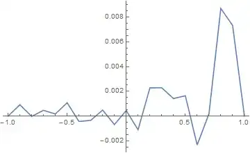
I don't know how your want to plot the two complex numbers (t vs c[t]).

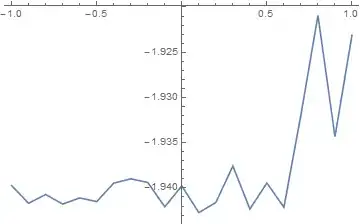
I chose to plot the real part of t on the x - axis and make two plots with the imaginary part of c[t] on the y -axis.

ListLinePlot[Transpose[{Re[solT1[[All, 1]]], Im[cList[[All, 2]]]}]]

ListLinePlot[Transpose[{Re[solT1[[All, 1]]], Re[solT1[[All, 2]]]}]]