Solve motion from Hamilton's equations

Question

I have a system of four coordinates and four momenta (conjugates of coordinates).

I have a metric tensor $g_{ik}$ and I know the Hamiltonian:

$H(p,q,t)=\frac{1}{2}g^{ik}(q)p_ip_k$

For my current case I have the Schwartzschild metric:

$ds^2=(1-r_s/r)dt^2-\frac{1}{1-r_s/r}dr^2-r^2d\theta^2-r^2sin^2(\theta)d\phi^2$

Meaning, the Hamiltonian is:

$H=\frac{1}{2}[\frac{1}{1-r_s/r}p_t^2-(1-r_s/r)p_r^2-\frac{1}{r^2}p_\theta^2-\frac{1}{r^2sin^2(\theta)}p_\phi^2]$

As Mathematica code with $r_s = 1$,

h =  1/2 (1/(1 - 1/r) pt^2 - (1 - 1/r) pr^2 - 1/r^2 pθ^2 - 1/(r^2 Sin[θ]^2) pϕ)

The equations of motion by Hamilton's equations are:

$dt/d\tau=\frac{\partial H}{\partial p_t};$

$dr/d\tau=\frac{\partial H}{\partial p_r};$

$d\theta/d\tau=\frac{\partial H}{\partial p_\theta};$

$d\phi/d\tau=\frac{\partial H}{\partial p_\phi};$

$dp_t/d\tau=-\frac{\partial H}{\partial t};$

$dp_r/d\tau=-\frac{\partial H}{\partial r};$

$dp_\theta/d\tau=-\frac{\partial H}{\partial \theta};$

$dp_\phi/d\tau=-\frac{\partial H}{\partial \phi};$

And I want to solve these equations of motion. I've tried deriving the expressions for each partial derivatives of $H$ and then substituting them in these equations manually. However, is there any way to do this dynamically?

What I mean is: suppose, we've only got the expression of Hamiltonian:

$H=H(p_t,p_r,p_\theta,p_\phi,t,r,\theta,\phi)$

And I want to dynamically derive all the partial derivatives and construct system of 8 (in this case) first-order differential equations and then solve them with NDSolve[]. So, that next time, when I want to try something else, all I have to change is the Hamiltonian.

P.s.: I've tried lots of things, like using Function[] for Hamiltonian and throwing variables back and forth, but with no effective result.

Did you look at NDSolve? (Or maybe DSolve?) If it's a separable Hamiltonian system (I didn't check), there are special integration methods available. See http://reference.wolfram.com/language/tutorial/NDSolveSplitting.html. — Michael E2, Dec 27 '15 at 19:40
I don't think it's separable (at least, at first sight, it's not... there are $r$ s everywhere). Yes, I've been fighting with NDSolve[] this whole time. My problem is, I can't differentiate $H$ partially so that it's analytic. Mathematica can't seem to understand that the variables of result functions (partial derivatives) are by themselves functions of $\tau$ and I don't know how to make it understand. — giochanturia, Dec 27 '15 at 19:46
I've posted an answer based on a function that I wrote earlier. To get a more specific answer regarding your exact problem with differentiation, it would be necessary for you to post the actual Mathematica code you've tried. — Jens, Dec 27 '15 at 19:59
After all my attempts failed, I erased them all and substituted the partial derivatives manually. Now I regret that, though... — giochanturia, Dec 27 '15 at 20:05
My codes, however, were not half as complex as yours is. I'll have to study it carefully. Thanks for sharing, I appreciate it a lot. — giochanturia, Dec 27 '15 at 20:06

Jens · Accepted Answer · 2015-12-27T20:03:24.260

Here is a convenience function that I use to solve for the motion under arbitrary classical Hamiltonians:

hamiltonSolve[hamilton_, varList_] := Module[
  {inputVariables, initialValues, phaseSpace, t, tMax, localH},
  {t, tMax} = Last[varList];
  {inputVariables, initialValues} = Transpose[Most[varList]];
  phaseSpace = Through[inputVariables[t]];
  localH = hamilton /. Thread[inputVariables -> phaseSpace];
  inputVariables /. First[
    NDSolve[
     Join[Thread[
       D[phaseSpace, t] == Flatten[
         Reverse[{-1, 1}*Partition[
            D[localH, {phaseSpace}], Length[phaseSpace]/2
            ]]
         ]],
      Thread[(phaseSpace /. t -> 0) == initialValues
       ]],
     inputVariables,
     {t, 0, tMax},
     MaxSteps -> Infinity]
    ]
  ]

sol = hamiltonSolve[
  1/2 (1/(1 - 1/r) pt^2 - (1 - 1/r) pr^2 - 1/r^2 pθ^2 - 1/(r^2 Sin[θ]^2) pϕ), 
   {{t1, 0.1}, {r, 2}, {θ, 0.1}, {ϕ, 0}, 
    {pt, 1}, {pr, .1}, {pθ, 0}, {pϕ, .1}, {t, 10}}];

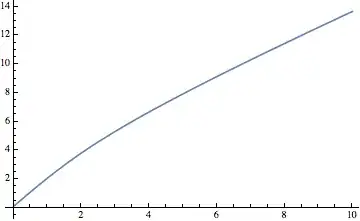
This provides all solutions as InterpolatingFunction objects which can be plotted. For example, here is the time as a function of proper time (I copied your Hamiltonian and set $r_s=1$):

Plot[sol[[1]][t],{t,0,10}]

The Hamiltonian is provided as the first argument of hamiltonSolve, and the second argument is a list of all the canonical variables with their initial values. As its last argument, the list additionally contains the name of the proper time variable (here I just call it t because it doesn't appear in the Hamiltonian anyway), together with the desired duration of the integration. The list of canonical variables must be even, and it is assumed that the canonical momenta are listed as the second half of the list (excluding the proper time).

So the list varList is generally of the form

{{x, x0}, {y, y0}, ... , {px, px0}, {py, py0}, ..., {t, tMax}}.

where in your case I entered the time t1 as the first coordinate, so that the corresponding momentum pt is the fifth entry in the list above.

I wanted to use your Code for my problem but very hard to understand how you construct hamiltonSolve[...]. My Hamilton function is: -0.2 II[t] m1[t] (1 - 0.18 n0[t])^2 SS[t] + m2[t] (-0.02 II[t] + 0.2 II[t] (1 - 0.18 n0[t])^2 SS[t]) + 0.97 (-0.65 II[t] - SS[t] + n0[t] (II[t] + SS[t]))^2 and co-state vars are m1[t], m2[t] and my state variables are SS[t], II[t] and control variable is n0[t]. Initial values: SS[0]=.97, II[0]=.02, m1[0]=2, m2[0]=10. Can you run your function using these parameters? Also, I do not understand why you have {t1, .1} in your function. — Tugrul Temel, Dec 23 '20 at 00:44

Solve motion from Hamilton's equations

1 Answers1

Linked