Plotting a function with insight to a special plot

Question

I draw this plot:

Plot3D[Sin[x] Cos[y], {x, 0, 4 \[Pi]}, {y, 0, 4 \[Pi]}]

the default setting of Mathematica 10. results in the below plot:

At the first I don't know why the z axes is inverse! and what change must I do to replot the above one to have a shape same as below (however the below shape created by Matlab)

Specially the ellipsoids in xy plate and meshes!!!

I don't reproduce your plot, I get the z-axis to work the right way, version 10.3 http://i.imgur.com/cK8zoqr.png — Jason B., Jan 12 '16 at 11:34
For the plot at the bottom, try the example here: http://mathgis.blogspot.de/2010/11/color-coded-contour-lines-with.html, or the solution given here: http://mathematica.stackexchange.com/a/101926/9490 — Jason B., Jan 12 '16 at 12:06
My answer, which I was typing while JasonB commented, is similar to some of the links he gives. — Kellen Myers, Jan 12 '16 at 12:11
The Matlab plot is not the same function as the Mathematica plot. If you really meant "same," when you said "a shape same as below," you'll need to figure out what function you plotted in Matlab. — Michael E2, Jan 12 '16 at 12:25
Yes functions are not similar, Just the configuration and visualization was important to me. — Unbelievable, Jan 12 '16 at 13:47

score 4 · Accepted Answer · answered Jan 12 '16 at 12:07

First, let's get the colors right:

Plot3D[
 Sin[x] Cos[y], {x, 0, 4 Pi}, {y, 0, 4 Pi},
 ColorFunction -> Function[{x, y, z}, ColorData["Rainbow"][z]]
]

That one is easy enough. If you really want it to look like a mesh, that's not so easy. I don't know of an option that colors mesh as flexibly as it normally colors the plot in question. I'd recommend a cheap hack like making up a list lie this:

t = 0.03;
myRanges = Map[# + {-t, t} &, Range[0, 4 Pi, Pi/8]];
myRanges[[1, 1]] = 0; myRanges[[-1, -1]] = 4 Pi;
myRanges = Interval @@ myRanges;

and then including the option as follows:

Plot3D[
 Sin[x] Cos[y], {x, 0, 4 Pi}, {y, 0, 4 Pi},
 ColorFunction -> Function[{x, y, z}, ColorData["Rainbow"][z]],
 RegionFunction -> Function[{x, y, z},
  IntervalMemberQ[myRanges, x] || IntervalMemberQ[myRanges, y]],
 PlotPoints -> 150
]

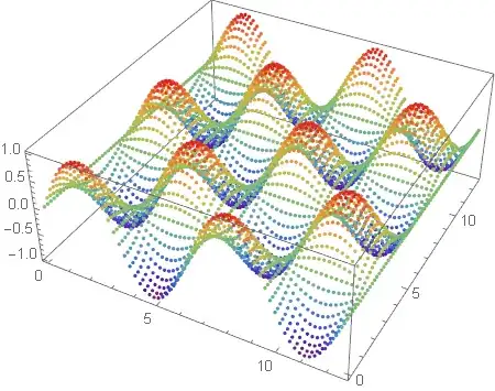
Not a great method, considering the PlotPoints required. Another alternative would be a 3D list plot to get a similar discrete effect, like the following:

ListPointPlot3D[
 Flatten[Table[{x, y, Sin[x] Cos[y]},
  {x, 0, 4 Pi, Pi/16}, {y, 0, 4 Pi, Pi/16}], 1],
 ColorFunction -> Function[{x, y, z}, ColorData["Rainbow"][z]]
]

Now, I'm not sure this is an important diversion. There are probably half a dozen other ways to get a similar effect, some of which are better than the two I've offered.

All that aside, there is a function called SliceContourPlot3D. This is the key to getting what you want. You can obtain the regions you want with:

SliceContourPlot3D[Sin[x] Cos[y],
 z == 0,
 {x, 0, 4 Pi}, {y, 0, 4 Pi}, {z, -1, 1}
]

This gives you a 2D contour plot in 3D, where the contour is drawn on the surface defined by the second argument. Now, we just want to bump it down to z=-2 (important: and change the z range accordingly) and change the style, to give your final output:

Show[
 Plot3D[Sin[x] Cos[y], {x, 0, 4 Pi}, {y, 0, 4 Pi},
  ColorFunction -> Function[{x, y, z}, ColorData["Rainbow"][z]],
  PlotStyle -> Opacity[0.7]
 ],
 SliceContourPlot3D[Sin[x] Cos[y],
  z == -2,
  {x, 0, 4 Pi}, {y, 0, 4 Pi}, {z, -3, 1},
  Contours -> Table[
   {t, ColorData["Rainbow"][(t + 1)/2]}, {t, -1, 1, 0.2}
  ],
  ContourShading -> None
 ],
 PlotRange -> All
]

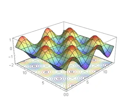
I also added some opacity to the plot as well. Note that you have to specify the contours explicitly (which I've done in the table) in order to individually modify their colors.

One last remark, the function you've plotted in MatLab does not appear to be the same one you give for plotting in Mathematica. I assume you know this.

Plotting a function with insight to a special plot

1 Answers1

Linked