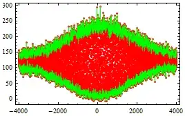
I have an experimental data from Michelson interference and I can fit the envelope in OriginPro9.0 using Global Fitting with shared parameters. The figure by OriginPro9.0 is like this:
However, I hope to realize this function in Mathematica. Here is what I did in Mathematica:
The source data is here.
Firstly, I smooth the up envelop and down envelop.
SetDirectory[NotebookDirectory[]];
name = "MichelsonInterference.txt";
b = Import[name, "Table"];
xmin = Min[b[[All, 1]]]; xmax = Max[b[[All, 1]]]; ymin = Min[b[[All, 2]]]; ymax = Max[b[[All, 2]]];
wd = 3; (*window width for average*)
step = 3;(*scan step in x, from xmin to xmax with the step*)
windowMin[data_, w_][pt_] := {pt, Min[Cases[data, {x_, y_} /; pt - w <= x <= pt + w][[All, 2]]]}
windowMax[data_, w_][pt_] := {pt, Max[Cases[data, {x_, y_} /; pt - w <= x <= pt + w][[All, 2]]]}
upenv = Table[windowMax[b, wd][t], {t, xmin, xmax, step}];
downenv = Table[windowMin[b, wd][t], {t, xmin, xmax, step}];
fig1 = ListLinePlot[b, PlotRange -> All, PlotStyle -> {Red}, Joined -> False, Frame -> True, Axes -> False];
fig2 = ListLinePlot[{upenv, downenv}, PlotRange -> All, Axes -> False,  Frame -> True, PlotStyle -> {{Green, Thin}, {Green, Thin}}];
Show[fig1, fig2]
The result is here:
Secondly, I try to fit the up envelop and down envelop with the same parameters {y0, xc, w}, but different A, using the method introduced here.
data1 = upenv;
data2 = downenv;
Remove[f, y0, A, w, xc];
f[x_, A_, y0_, xc_, w_] := y0 + A/(w Sqrt[π/2])*Exp[-2*((x - xc)/w)^2];
x0 = (xmin + xmax)/2; h = ymax; Δx = (xmax - xmin)/4;
vars = {{y0, 0}, {xc, x0}, {w, Δx/2}, {A1, h*Δx/2}, {A2, -h*Δx/2}};
logModel = -Total[(data1[[All, 2]] - (f[#, A1, y0, xc, w] & /@
    data1[[All, 1]]))^2]/2 - Total[(data2[[All, 2]] - (f[#, A2, y0, xc, w] & /@ data2[[All, 1]]))^2]/2;
fit = FindMaximum[logModel, vars]
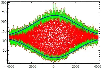
With these fitted values, I plot all the figures together.
Show[ListLinePlot[b, PlotRange -> All, Joined -> False, PlotStyle -> {Red, Thin}], ListLinePlot[{upenv, downenv}, PlotRange -> All, Axes -> False, Frame -> True, PlotStyle -> {{Green, Thin}, {Green, Thin}}], Plot[ 121.6 + 551180/(3927.6 Sqrt[π/2])*Exp[-2*((x - 95.64)/ 3927.6 )^2], {x, xmin, xmax}, PlotStyle -> {Blue, Thick}, PlotRange -> All], Plot[121.6 + -537445/(3927.6 Sqrt[π/2])* Exp[-2*((x - 95.64)/ 3927.6 )^2], {x, xmin, xmax}, PlotStyle -> {Blue, Thick}, PlotRange -> All],Axes -> False, Frame -> True, AspectRatio -> .67, LabelStyle -> Directive[Black, Medium], ImageSize -> {300, 200}]
The final result by Mathematica is
My problem is that this fitted figure by Mathematica is different from the one by OriginPro9.0 (the first figure). I hope to obtain the same result as what I got in OriginPro9.0. For example, the FWHM of figure by Mathematica should be narrower. Could you help me by improving my Mathematica codes? Thank you all in advance!


It seems that approx. in Origin was done for unfiltered data..
– Rom38 Jan 20 '16 at 07:46