Fitting a spline to data with FindFit?

Question

I am trying to find a function that fits my almost linear data. A high order polynomial model has too much residual. So I was hoping to use Mathematica to fit splines to the curve.

This is what I would like to see in an example.

FindFit with a spline function
How to get model stats like what LinearModelFit provides.
How to dump the spline terms and control points so I can implement in "C"

I can then use the cubic spline on my embedded platform.

So can I get a symbolic representation of this function so I can implement it?

You can get the sample data here

Do you need a fit or an interpolation? You're using both terms, but they aren't the same. — Sjoerd C. de Vries, Sep 11 '12 at 21:29
Welcome to Mathematica.SE by the way. Of Dutch descend, by any chance? — Sjoerd C. de Vries, Sep 11 '12 at 21:31
can we have a sample of your data? is it only y-values or {x,y} pairs? Full data would be much better. And do you need the fit curve to pass exactly through all points or just reflect on general trend? — Vitaliy Kaurov, Sep 11 '12 at 23:14
The function just needs to reflect a trend. I added a link to the data. It is just {x,y} pairs. — witkamp, Sep 11 '12 at 23:29
Are you sure they are {x,y} and not {y,x}? I mean: the integers are y values? — Dr. belisarius, Sep 12 '12 at 00:21
You might like to have a look at BSplineCurve: http://reference.wolfram.com/mathematica/ref/BSplineCurve.html#30165982 — Oleksandr R., Sep 12 '12 at 18:32
@OleksandrR. Thanks for the link. It was exactly what i wanted. I never thought of looking there because I thought of BSplineCurve as only a graphics function. — witkamp, Sep 13 '12 at 16:20
@witkamp yes, it's strange that these examples are on the BSplineCurve documentation page rather than the one for BSplineBasis. To get the goodness-of-fit statistics you can probably use BSplineBasis with LinearModelFit rather than constructing the design matrix manually as shown in the example. I'd have posted an answer except I wasn't sure if that was what you were looking for and haven't used splines for anything before, so I have no real familiarity with them. Please feel free to self-answer if you like. — Oleksandr R., Sep 14 '12 at 01:04
Strongly related: "Implementation of smoothing splines function," "How to make BSplineFunction pass each data point and naturally smooth?" — Alexey Popkov, Oct 23 '13 at 15:17
It amazes me this is such a highly voted question with a highly voted answer that does not answer the question an arbitrary polynomial is not a spline. — george2079, Mar 23 '18 at 20:25
@george2079, I agree! I just need the correct answer to accept! — witkamp, Oct 31 '19 at 20:26

Vitaliy Kaurov · Answer 1 · 2012-09-12T00:36:24.087

6

Taking your data in account from link you provided:

data={{......}};

Find the model:

model = Fit[data, x^# & /@ Range[0, 10], x]

20.2513 + 43.3389 x - 0.208411 x^2 + 0.193888 x^3 - 0.0341689 x^4 + 
 0.00281455 x^5 - 0.000131003 x^6 + 3.64629*10^-6 x^7 - 
 6.01724*10^-8 x^8 + 5.43205*10^-10 x^9 - 2.06702*10^-12 x^10

Verify it is more or less correct:

Show[ListPlot[data, PlotStyle -> Directive[PointSize[.02], Opacity[.02], Red]], 
 Plot[model, {x, -7, 55}, PlotStyle -> Thickness[.005]], 
 Frame -> True, Axes -> False, ImageSize -> 500]

enter image description here

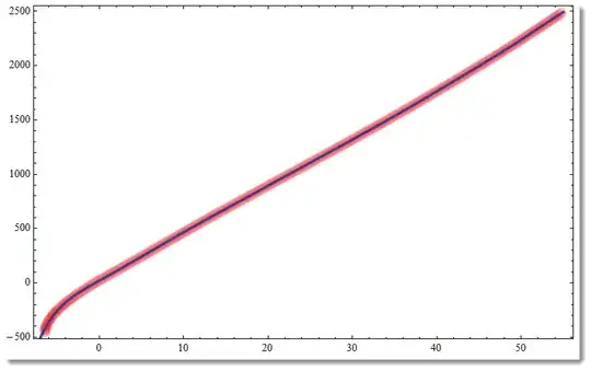
The blue line inside is your model. Red line is your data points blended together (too many of them) with applied opacity. I've chosen so many polynomial terms to take in account well little bent at the beginning. You can play with number of polynomial terms.

Export your model to C:

CForm[model]

20.251253486790134 + 43.33892854755122*x - 0.20841104603541305*Power(x,2) + 
   0.19388822209706186*Power(x,3) - 0.03416888859439315*Power(x,4) + 
   0.0028145533596680857*Power(x,5) - 0.0001310033312242676*Power(x,6) + 
   3.646291289683582e-6*Power(x,7) - 6.017238075935027e-8*Power(x,8) + 
   5.432049184033492e-10*Power(x,9) - 2.0670190082996488e-12*Power(x,10)

edited Sep 12 '12 at 00:36

answered Sep 11 '12 at 23:47

Vitaliy Kaurov

73,078
9
204
355

Just in case this works much better for the left "tail" f[x_]:=24.9*x + 2.206*x*Sin@x + x^2*Sin@x + Tan[0.2407*x] - 5.611*x^2 – Dr. belisarius Sep 12 '12 at 00:11
3

If you're expecting to be doing high-order polynomial fits, I would recommend using LinearModelFit[], taking one basis function at a time, and monitoring the value of "AdjustedRSquared" to guard against overfitting (or use the fancier methods, such as cross-validation). – J. M.'s missing motivation Sep 12 '12 at 01:35
@belisarius Ahh, what's the name of the program you used to get this expression? The one that fits models of different complexity to the data... – Ajasja Sep 12 '12 at 08:50
1

@Ajasja, Eureqa? – J. M.'s missing motivation Sep 12 '12 at 10:43
@J.M. The name is Formulize now. And they now sell cloud time for parallel evaluations. – Dr. belisarius Sep 12 '12 at 11:33
@belisarius I just downloaded it. Very cool program. User friendly too. I wonder how it compares to the commercial Mathematica 'equivalent' at http://www.evolved-analytics.com/ – Sjoerd C. de Vries Sep 12 '12 at 11:52
@J.M. Thanks for pointing me to that program. Very interesting. Reminds me of this answer of mine. – Sjoerd C. de Vries Sep 12 '12 at 12:02
@SjoerdC.deVries My experiments with Formulize gave me both good and bad results. If you do know a few things about the model, you can inject that knowledge into the software in several (sometimes subtle) ways. It is sometimes very slow to converge to a good solution, but I never bought real computing power (a cloud grid) to be serious about this complain. – Dr. belisarius Sep 12 '12 at 12:10
@belisarius That's the one I had in mind. Thanks. – Ajasja Sep 12 '12 at 12:27
3

The residuals for the 12th order polynomial are too high. That is why I would like to fit a SPLINE to the curve. Also this needs to be implemented on an embedded platform with software FP. – witkamp Sep 12 '12 at 17:14
@witkamp, with what you've just said, I'm not even entirely sure that a smoothing spline is the best way to go about it. As a start, could you edit your question to talk a bit about the provenance of your data? – J. M.'s missing motivation Sep 13 '12 at 02:54
@witkamp once you found a spline fit, like this or like this how do you intend to port it to C ? It is still in Mathematica intrinsic form. Won't you have exactly same problem as you had with InterpolatingFunction? – Vitaliy Kaurov Sep 13 '12 at 03:16
@J.M. I added a comment above about a spline. – Vitaliy Kaurov Sep 13 '12 at 03:18
@J.M The data table maps mV to Deg F. for a k-Type Thermocouple. – witkamp Sep 13 '12 at 16:17
@VitaliyKaurov I would implement the BSplineBasis function in C use it to calculate the spline. – witkamp Sep 13 '12 at 16:19
@J.M. What other methods would you recommend? – witkamp Sep 13 '12 at 16:25
As I said @witkamp, please edit that information into your question... – J. M.'s missing motivation Sep 13 '12 at 22:31

Fitting a spline to data with FindFit?

1 Answers1