Numerical Differentiation using 1500 data points

Question

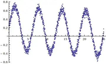
I have a set of 1500 data points (which are some energy eigenvalues) corresponding to a parameter H0 (which represents magnetic field. H0 values are equispaced going from $-3.0$ to $3.0$ in steps of $0.005$. Please note that the energy eigenvalues are not exact and they have experimental error in them. What I am trying to do is first plot those data points in Mathematica.

I have found the command ListLinePlot[{{x1, y1}, {x2, y2}, ...}]. However, feeding such a huge set of data points consumes a lot of time. So is there any other way out? For example, importing the data file from Fortran. I have used the command Import["file", "table"] where "file" is a Fortran data file. But it is giving the error message "File not found during import".

Then I would like to find the second derivative of the plot. Accurate evaluation of second derivative is very crucial for my purpose. I have done the plot using "gnuplot" and then found the first derivative of the plot using the central difference formula: $\frac{f(x+h)-f(x-h)}{2h}$. Here $h = 0.005$. Then I evaluated the first derivative of the latter plot using the same formula to get the second derivative plot.

I am getting the plot but not the desired result (a peak is to be obtained near a value of H0, pre-calculated). In other words, I am getting a disagreement between theoretical and numerical values of H0. The eigenvalue evaluation is OK I think because I have checked it both in Mathematica and Fortran. Maybe something is going wrong in the second derivative evaluation. Kindly advise how to carry out numerical differentiation from a set of data points in Mathematica.

Answer 1

There is a Fourier transform method here. Using the example from belisarius it might be done as below. Caveat: I do not guarantee I made no cut-and-paste errors. Your mileage may vary. Considerably.

(* sample data *)
g[x_] := x + 1/2 Sin[x] + RandomVariate[NormalDistribution[.2, .05]];

SeedRandom[1111];
xmax = 8*Pi;
nHalf = 750;
n = 2*nHalf;
xt = Table[i*xmax/n, {i, 0, n}]; (* the domain sampling points *)
t = Table[g[x], {x, 0., 8. Pi, xmax/n}];

(* Subtract beginning from end to get drift; we need to remove that to get something that is periodic-like. Probably should average the first few and last few points to get a better approximation to the drift. *)

range = t[[-1]] - t[[1]];

t2 = t - Range[Length[t]]*range/Length[t];

(* Smoothing magic...*)
ismooth = 10;

(* Get FT, multiply appropriately to get FT of derivative, then invert by IFT. last, add back the linear drift. *)

fourier = Fourier[t2];
freq1 = -2*Pi*I*
  Table[i*Exp[-(i/ismooth)^2], {i, 1, nHalf}]/(xmax);
freq2 = 
 2*Pi*I*Table[i*Exp[-(i/ismooth)^2], {i, 1, nHalf}]/(xmax);
freq = Join[{0}, freq1, Reverse[freq2]];
fourierd = fourier*freq; 
der = InverseFourier[fourierd] + range/xmax;

(* Pictures *)
ListPlot[Transpose[{xt, t}]]

(* Plot of samples minus drift *)
ListPlot[Transpose[{xt, t2}], PlotStyle -> {Thickness[0.001]}]

(* approximated derivative *)

ListPlot[Transpose[{xt, der}], PlotStyle -> {Thickness[0.001]}

(* We can get the second derivative similarly. Since we used a linearized approximated drift we need not add it back at the end.*)

freq1b = (-2*Pi*I)^2*
   Table[i^2*Exp[-(i/ismooth)^2], {i, 1, nHalf}]/xmax^2;
freq2b = (2*Pi*I)^2*
   Table[i^2*Exp[-(i/ismooth)^2], {i, 1, nHalf}]/xmax^2;
freqb = Join[{0}, freq1b, Reverse[freq2b]];
fourierd2 = fourier*freqb;
der2 = InverseFourier[fourierd2];

ListPlot[Transpose[{xt, der2}], PlotStyle -> {Thickness[0.001]}]

I also tried this with

g2[x_] := Exp[x^(1/10)] - Exp[-x^2*Abs[Cos[x]]] + 
   RandomVariate[NormalDistribution[.2, .05]];

I got what I believe were tolerable results, although maybe not useful at the ends. No surprise, given that this is not so close to "periodic plus linear drift".

Answer 2

Here is a way that combines two filters and a numerical eighth order approximation to the derivatives. Depending on your data, it may work pretty well.

Another (perhaps better) alternative is using a Savitzky-Golay style filter.

Some code:

(* Derivative Coeffs *)
ld = With[{m = 1, s = 8, n = 16}, CoefficientList[Normal[Series[x^s Log[x]^m, {x, 1, n}]], x]]
g[x_] := x + 1/2 Sin[x] +  RandomVariate[NormalDistribution[.2, .05]]; 
(*Our data*)
t = Table[g[x], {x, 0, 8 Pi, 8 Pi/1500}];
(*filtered data*)
tvf = TotalVariationFilter[t, 20, MaxIterations -> 100]
(* First derivative*)
fd = ListCorrelate[ld, MovingAverage[tvf, 30]];
(*second derivative*)
sd = MovingAverage[ListCorrelate[ld,TotalVariationFilter[fd, 20, MaxIterations -> 100]], 20];
GraphicsGrid[{ListPlot /@ {t, tvf}, ListPlot /@ {fd, sd}}]

Answer 3

Depending on the data, you may be able to use the built-in DerivativeFilter to locate the peak in the second derivative.

Create some noisy example data with a pronounced peak in the second derivative:

data = Table[
   1 - TriangleWave[x] + RandomReal[NormalDistribution[0, .05]], 
  {x, 0, 0.5, 0.5/1500.}];

Use a DerivativeFilter with a large value for the regularization parameter:

smoothedSecondDerivative = DerivativeFilter[data, {2}, 50.];

This produces a rather wide peak, but it may be good enough to locate the position of the peak. For data with a higher SNR you could use a smaller regularization parameter and obtain a narrower peak.

ListLinePlot[{data, 50000 smoothedSecondDerivative}, PlotRange -> All]

Answer 4

You can use Interpolation to create an InterpolationFunction and then perform the derivation on the interpolation function:

data = Table[{x, Cos[x]}, {x, 0, 2 Pi, 0.01}];
fkt = Interpolation[data];
Plot[{fkt[x], fkt'[x]}, {x, 0, 2 Pi}]

The prime (fkt') gives you the first derivative. Alternatively you can use D[fkt[x], x]