Calculus 1: Create the plot of a function satisfying certain conditions

Question

Today in class we were shown how to create an infinite limit graph (plot) given the preceding conditions. While I have a fairly terrible sketch of this graph in my notebook, I'd like to create a clean version with Mathematica to import into my notes.

Here were the conditions:

$$ \begin{align*} g(2)&=1\\ g(5)&=-1\\ \lim_{x\to4}g(x)&=-\infty\\ \lim_{x\to-7^-}g(x)&=\infty\\ \lim_{x\to-7^+}g(x)&=-\infty\\ \end{align*} $$

Any help would be appreciated!

Answer 1

g[x_] := 1/Abs[x - 4] + 1/(x + 7);
sol = Solve[a g[2] + b  == 1 && a g[5] + b == -1, {a, b}];
g1[x_] := (a g[x] + b) /. sol; 
Plot[g1[x], {x, -12, 8}, Evaluated -> True, 
     Epilog -> {Red, PointSize[Medium], Point[{{2, 1}, {5, -1}}]}]

Edit

How to build these kind of things?

Answering the comments by the OP, I'll try to sketch up how one can build up this kind of functions.

First thing to note is that you can construct a divergence at $x_0$ simply by

$f(x) = \frac1{x-x_0}$ or $f(x) = \left|\frac1{x-x_0}\right|$ depending on the type of divergence you want to get. Let's see one example:

GraphicsGrid[
  Table[Framed@
           Plot[sign f, {x, -2, 2}, PlotRange -> {{-2, 2}, {-4, 4}}, 
                PlotLabel -> Style[Framed[sign f], 11, Blue, Background -> Lighter[Yellow]]],
  {sign, {-1, 1}}, {f, {1/(x - 1), 1/Abs[x - 1]}}]]

Now, by adding up two of those, with different poles, we get a function with two divergences, like the one posted above. Let's see another example of that:

Framed@Plot[1/(x - 1) + 1/(x - 3), {x, -1, 4}]

See? We got our function with two divergences at x = {1, 3}.

But you still have an additional requirement, because your function has two clamped values.

$$ \begin{align*} g(2)&=1\\ g(5)&=-1\\ \end{align*} $$

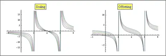
For doing that we add two degrees of freedom to the function: a scale (elongation) and an offset. Let's see what kind of things we can do with that:

Framed@GraphicsRow@{
  Plot[Table[a (1/(x - 1) + 1/(x - 3)), {a, 1, 3, .5}], {x, -1, 4}, 
    Evaluated -> True, 
    PlotLabel -> Style[Framed[Scaling], 14, Blue, Background -> Lighter[Yellow]]],
  Plot[Table[a + 1/(x - 1) + 1/(x - 3), {a, 1, 3, .5}], {x, -1, 4}, 
    Evaluated -> True, 
    PlotLabel -> Style[Framed[Offsetting], 14, Blue, Background -> Lighter[Yellow]]]}

The way to add that freedom is to build a new function with two additional parameters a and b.

$g(x) =\frac{a}{(x-3) (x-1)}+b$

However, although it's easy, I'm not going to demonstrate here that by doing this, and finding appropriate values for a and b, which is the objective of our Solve[] trick in the original incarnation of this answer, you can clamp any two values. Do it as an exercise!

(Hint:

sol = Solve[a g[x0] + b == y0 && a g[x1] + b == y1, {a, b}]

)

Some food for thought

If you want to investigate it further, you can think why the following is able to clamp three points. Please note the function is not squared but cubed below ... and think Why? :

f[x_] := 1/Abs[x - 4] + 1/(x + 7);
g[x_] := a f[x]^3 + b f[x] + c
sol = Solve[g[2] == 1 && g[5] == -1 && g[-10] == 0, {a, b, c}];
g1[x_] := g[x] /. sol;
Framed@Plot[g1[x], {x, -12, 8}, Evaluated -> True, 
  PlotRange -> {{-12, 7}, {-4, 4}},
  Epilog -> {Red, PointSize[Medium], Point[{{2, 1}, {5, -1}, {-10, 0}}]}]