Why does repeating an equation help in FindRoot?

Question

I'm trying to understand this behavior of FindRoot. Consider a sample function (the one I'm actually interested in is far more complicated, but has similar issues) and the following arguments:

crazyFunction[x_, y_] := N@Norm[{x + 2 y}]
yact = RandomReal[{-10, 10}, 2]~Join~{RandomReal[{100, 250}]};
gv = yact + RandomReal[{-.1, .1}, 2]~Join~{RandomReal[{-5, 5}]};
sampledata = crazyFunction[#, {a, b, c}] == crazyFunction[#, yact] & /@
 {{1, 2, 3}, {2, 3, 4}, {4, 5, 6}};

Basically, I'm applying the sample function for a particular yact value, at three x values, and setting it equal to the function evaluated with three "unknown" y values {a,b,c}. To solve for the "unknown" values, I used FindRoot with initial guessed value gv randomly perturbed from the actual values:

sol = FindRoot[sampledata, Transpose@{{a, b, c}, gv}, MaxIterations -> 1000]

Note, this likely will throw a warning (* FindRoot::lstol: The line search decreased the step size to within tolerance specified by AccuracyGoal and PrecisionGoal ... *).

To evaluate the quality of the solution, I compare the Norm of the difference between the actual yact and the solved y (normalized to the Norm of yact):

Norm[yact - {a, b, c} /. sol]/Norm[yact]
(* Out[]:= 0.0540657 *)

which isn't a terrible value.

My thinking here is, I have three unknowns -- a, b, and c -- and three different equations for the different x values, so that should be enough to solve the problem. In fact, without three equations FindRoot won't work. I.e.:

FindRoot[sampledata[[1]], Transpose@{{a, b, c}, gv}, MaxIterations -> 1000]
(* FindRoot::nveq: The number of equations does not match the number of variables in... *)

But, if instead of using three, different equations, I simply repeat the same equation three times:

sampledata = Table[crazyFunction[#, {a, b, c}] == crazyFunction[#, yact] &@{1, 2,3}, {3}];
sol = FindRoot[sampledata, Transpose@{{a, b, c}, gv}, MaxIterations -> 1000];

Not only does it not give the lstol warning, but it actually gets a more accurate result! Consider:

dat=Table[yact=RandomReal[{-10,10},2]~Join~{RandomReal[{100,250}]};
 gv=yact+RandomReal[{-.1,.1},2]~Join~{RandomReal[{-5,5}]};
 sampledata=crazyFunction[#,{a,b,c}]==crazyFunction[#, yact]&/@{{1,2,3},{2,3,4},{4,5,6}};
 sol=Quiet@FindRoot[sampledata,Transpose@{{a,b,c},gv},MaxIterations->1000];
 Norm[yact-{a,b,c}/.sol]/Norm[yact],{1000}];

datSamedata=Table[
 yact=RandomReal[{-10,10},2]~Join~{RandomReal[{100,250}]};
 gv=yact+RandomReal[{-.1,.1},2]~Join~{RandomReal[{-5,5}]};
 sampledata=Table[crazyFunction[#,{a,b,c}]==crazyFunction[#, yact]&@{1,2,3},{3}];
 sol=Quiet@FindRoot[sampledata,Transpose@{{a,b,c},gv},MaxIterations->1000];
 Norm[yact-{a,b,c}/.sol]/Norm[yact],{1000}];

Histogram[{dat, datSamedata}, "Log"]

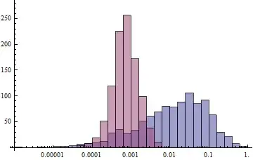
Note the log-binning. Using the same equation three times is far more accurate than using three different equations!

So, my question is: Why is repeating the same equation three times far more accurate than using three different equations?

Answer 1

Here's one way to think about the 2D Newton's method, which explains why a 2D Newton's method applied to a redundant system can lead to the exact result after just one step. Some variant of this is likely used by FindRoot.

We want to find the roots of a two by two system. Start with an initial guess $(x_0,y_0)$, set up linear approximations to each equation, and solve the two by two linear system that results to improve the guess. Suppose, for example, we want the simultaneous roots of the following system.

f[x_, y_]  := x^3 - 2 y;
g[x_, y_]  := y^3 - 2 x;

It's easy to see that the solutions are $(x,y)=(0,0)$ or $(x,y)=(\pm\sqrt{2},\pm\sqrt{2})$.

Here's the general solution of the corresponding linear system.

fx[x_, y_] := D[f[x, y], x];
fy[x_, y_] := D[f[x, y], y];
gx[x_, y_] := D[g[x, y], x];
gy[x_, y_] := D[g[x, y], y];
{sol} = Solve[{
  f[x0, y0] + fx[x0, y0] (x - x0) + fy[x0, y0] (y - y0) == 0,
  g[x0, y0] + gx[x0, y0] (x - x0) + gy[x0, y0] (y - y0) == 0}, 
{x, y}];
sol

This suggests that we iterate the following function.

newt[{x_, y_}] = {
  (2*(3*x^3*y^2 + 2*y^3))/(-4 + 9*x^2*y^2),
  (2*(2*x^3 + 3*x^2*y^3))/(-4 + 9*x^2*y^2)
};
NestList[newt, {1.0, 1.0}, 5]

(* Out *)
{{1., 1.}, {2., 2.}, {1.6, 1.6}, {1.44225, 1.44225}, 
 {1.41501, 1.41501}, {1.41421, 1.41421}}

Looks good.

OK, now let's do it for a redundant system.

f[x_, y_]  := x^3 - 2 y;
g[x_, y_]  := x^3 - 2 y;

Any point of the form $(x,x^3/2)$ is a solution. Let's try Newton's method.

fx[x_, y_] := D[f[x, y], x];
fy[x_, y_] := D[f[x, y], y];
gx[x_, y_] := D[g[x, y], x];
gy[x_, y_] := D[g[x, y], y];
{sol} = Solve[{
  f[x0, y0] + fx[x0, y0] (x - x0) + fy[x0, y0] (y - y0) == 0,
  g[x0, y0] + gx[x0, y0] (x - x0) + gy[x0, y0] (y - y0) == 0}, 
 {x, y}];
sol

This suggests that we iterate the following function.

newt[{x_, y_}] = {x, x^3/2};

And we get to the exact solution after one step.