What is wrong with my code so it neither produces a correct plot nor an error message?

Question

I am trying to define some initial functions and then using them to define my secondary functions and then plot the secondary functions. I am supposed to get two curves with a finite width representing the uncertainty in the model parameter sets $\{a1, b1, c1\}$ and $\{a2, b2, c2\}$ corresponding to functions $CDDHybrid$ and $CDD40$ respectively while the other two functions $CDDNoterdaeme$ and $CDDZwaan$ have no uncertainties in their parameters. Below is my code:

CDDHybrid[s_, a1_, b1_, c1_] := 10^(a1 + b1*c1 - b1*s)*Exp[-10^(s - c1)];
CDDHybridmean[s_] := 10^(-4.9684 - 0.88*s)*Exp[-10^(s - 20.82)];
CDD40[s_, a2_, b2_, c2_] := 10^(a2 + b2*c2 - b2*s)*Exp[-10^(s - c2)];
CDD40mean[s_] := 10^(-11.0765 - 0.57*s)*Exp[-10^(s - 20.55)];
CDDNoterdaeme[s_] := 10^(4.2502 - 1.27*s)*Exp[-10^(s - 21.26)];
CDDZwaan[s_] := 10^(3.378 - 1.24*s)*Exp[-10^(s - 21.2)];

LHSHybridmean[s_?NumericQ] := NIntegrate[Log[10]*10^u*CDDHybridmean[u], {u, s, Infinity}] ;
LHSHybrid[s_, a1_, b1_, c1_?NumericQ] := NIntegrate[Log[10]*10^u*CDDHybrid[u, a1, b1, c1], {u, s, Infinity}] ;
LHS40mean[s_?NumericQ] := NIntegrate[10^u*Log[10]*CDD40mean[u], {u, s, Infinity}] ;
LHS40[s_, a2_, b2_, c2_?NumericQ] := NIntegrate[10^u*Log[10]*CDD40[u, a2, b2, c2], {u, s, Infinity}] ;
LHSNoterdaeme[s_?NumericQ] :=  NIntegrate[10^u*Log[10]*CDDNoterdaeme[u], {u, s, Infinity}] ;
LHSZwaan[s_?NumericQ] :=  NIntegrate[10^u*Log[10]*CDDZwaan[u], {u, s, Infinity}] ;

With[{a1 = Interval[-23.29 + .04 {-1, 1}], 
  b1 = Interval[0.88 + .04 {-1, 1}], 
  c1 = Interval[20.82 + .01 {-1, 1}], 
  a2 = Interval[-22.79 + .06 {-1, 1}], 
  b2 = Interval[0.57 + .07 {-1, 1}], 
  c2 = Interval[20.55 + .03 {-1, 1}]}, 
 LogPlot[{Min[LHSHybrid[s, a1, b1, c1]], LHSHybridmean[s], 
   Max[LHSHybrid[s, a1, b1, c1]], Min[LHS40[s, a2, b2, c2]], 
   LHS40mean[s], Max[LHS40[s, a2, b2, c2]], LHSNoterdaeme[s], 
   LHSZwaan[s]}, {s, 20.3, 23.1}, PlotRange -> {10^-35., 1.0}, 
  Filling -> {1 -> {3}, 4 -> {6}}, 
  FillingStyle -> {{Blue, Opacity[0.4]}, {Red, Opacity[0.4]}}, 
  PlotStyle -> {Blue, Blue, Blue, Red, Red, Red, Brown, Green, Thick},
   Frame -> True, 
  FrameLabel -> {Style["X[unit]", FontSize -> 26], Style["Y[unit]", FontSize -> 26]}, 
  FrameTicksStyle -> Directive[FontSize -> 26], 
  PlotLegend -> {Style["", 20], Style["Hybrid (2015)", 20], 
    Style["", 20], Style["", 20], Style["40 arcseconds(2015)", 20], 
    Style["", 20], Style["Noterdaeme (2009)", 20], 
    Style["Zwaan (2005)", 20]}]]

However, I am surprised that I am getting nothing out of it! Could any one see what is my mistakes?

Min[LHSHybrid[s, a1, b1, c1]] will not output anything meaningful because in the definition of LHSHybrid, c1 has to satisfy NumericQ. Interval gives False when you apply NumericQ. The same applies with all other functions in LogPlot that have a1, b1, etc. in them.
In addition, infinity should have a capital i as the first letter, or else it will be treated as a variable. Infinity means infinity, and infinity means a variable named "infinity". — JungHwan Min, May 23 '16 at 01:06
Thus, all of the functions in your LogPlot are not numeric, meaning nothing will be on the graph. — JungHwan Min, May 23 '16 at 01:13
In fact, I meant "Infinity" somehow in pasting the copied lines, I wrote it as "infinity." I removed $?NumericQ$ from the definition of the functions which have constant parameters. It still doesn't work. Do you have a suggestion? — Benjamin, May 23 '16 at 01:23
Even making all initial functions numeric in nature doesn't solve the problem. But I was able to plot another set of functions in which there were no integrations. So, what causes the problem is the introduction of integrations into my functions which I don't know how to handle. — Benjamin, May 23 '16 at 01:33
So the only workaround seems to be removeing $?NumericQ$ AND replacing $NIntegrate$ with $Integrate$. But that is taking forever to run not mentioning intermediate warnings. Again, thanks for your feedback. — Benjamin, May 23 '16 at 01:45
The four functions that only have s as input seems to work fine; try restarting the kernel. NumericQ is still a problem. Also, the problem with the functions involving Intervals is that NIntegrate cannot have Intervals in them. — JungHwan Min, May 23 '16 at 01:49
Are you expecting to get an Interval from NIntegrate? If so, there might be a workaround to this. — JungHwan Min, May 23 '16 at 01:55
Hi. I removed ?NumericQ all together and turned NIntegrate into Integrate. The code still runs hopelessly. Sure, I am expecting to get an interval from NIntegrate. — Benjamin, May 23 '16 at 02:00
I think you can make your own interval function to plot the results, see the answer below. — Jack LaVigne, May 24 '16 at 00:20

Jack LaVigne · Accepted Answer · 2016-05-24T14:17:07.640

Introduction

The first thing that I noticed is that the functional form for all of your CDD and LHS functions are identical.

I propose that rather than defining six functions for each, we define one function and change the input arguments to cover the various cases.

cdd[s_, a_, b_, c_] := 10^(a + b*c - b*s)*Exp[-10^(s - c)]

lhs[s_?NumericQ, a_?NumericQ, b_?NumericQ, c_?NumericQ] := 
 NIntegrate[Log[10]*10^u*cdd[u, a, b, c], {u, s, Infinity}]

Note that we use NumericQ for all of the input arguments to lhs. This will be required the results are plotted.

As an example, here is the output for the average parameters you had set for the first case

With[
 {
  a1 = -23.29,
  b1 = 0.88,
  c1 = 20.82,
  s = 20.3
  },
 {cdd[s, a1, b1, c1], lhs[s, a1, b1, c1]}
 ]
(* {1.08754*10^-23, 0.00291862} *)

Interval

The problem you were experiencing is that you wanted to use Interval but it was not accepted by NIntegrate so one was stuck.

The strategy will be to create all permutations of the average inputs parameters +/- their deltas and compute the minimum and maximum.

So for the first step, imagine that we have three parameters a, b and c and when their respective delta is subtracted we have the minus version, am, bm and cm.

We can get a list of all permutation of minus

Flatten[Outer[List, {a, am}, {b, bm}, {c, cm}], 2]
(* {{a, b, c}, {a, b, cm}, {a, bm, c}, {a, bm, cm}, {am, b, 
  c}, {am, b, cm}, {am, bm, c}, {am, bm, cm}} *)

Clearly we can perform the same operation for adding the delta.

Next we will define two functions that use lhs but compute the minimum of subtracting the delta values and the maximum of adding the delta values.

The case is covered where delta is zero for a particular parameter.

lhsMinus[s_?NumericQ, a_?NumericQ, da_?NumericQ, b_?NumericQ, 
  db_?NumericQ, c_?NumericQ, dc_?NumericQ] := Module[
  {
   aList,
   bList,
   cList
   },
  aList = If[da == 0, {a}, {a, a - da}];
  bList = If[db == 0, {b}, {b, b - db}];
  cList = If[dc == 0, {c}, {c, c - dc}];

  Min[Map[lhs[s, Sequence @@ #] &, 
    Flatten[Outer[List, aList, bList, cList], 2]]]
  ]

lhsPlus[s_?NumericQ, a_?NumericQ, da_?NumericQ, b_?NumericQ, 
  db_?NumericQ, c_?NumericQ, dc_?NumericQ] := Module[
  {
   aList,
   bList,
   cList
   },
  aList = If[da == 0, {a}, {a, a + da}];
  bList = If[db == 0, {b}, {b, b + db}];
  cList = If[dc == 0, {c}, {c, c + dc}];

  Max[Map[lhs[s, Sequence @@ #] &, 
    Flatten[Outer[List, aList, bList, cList], 2]]]
  ]

Plot

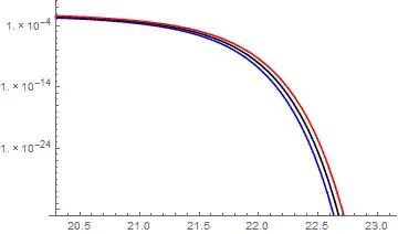
Now plot the results for the first set of parameters. For the large spread in the s values the delta's had to be increased or the min and max were too close to be visible.

With[
 {
  a1 = -23.29,
  da = 0.08,
  b1 = 0.88,
  db = 0.08,
  c1 = 20.82,
  dc = 0.04
  },
 LogPlot[
  {
   lhsMinus[s, a1, da, b1, db, c1, dc],
   lhs[s, a1, b1, c1],
   lhsPlus[s, a1, da, b1, db, c1, dc]
   },
  {s, 20.3, 23.1},
  {PlotStyle -> {Blue, Black, Red}},
   PlotRange -> {10^-35, 1}
  ]
 ]

Mathematica graphics

I think this should get you started. I leave to you the plot of the second data set.

Numerical Derivatives and a faster version

If one were able to ascertain the polarity that a change in a parameter has on the outcome one could construct a faster version by reducing the number of permutations.

testDeriv = With[
  {
   a1 = -23.29,
   b1 = 0.88,
   c1 = 20.82
   },
  Table[
   {s, (lhs[s, a1 + 0.001, b1, c1] - lhs[s, a1, b1, c1])/0.001,
    (lhs[s, a1, b1 + 0.001, c1] - lhs[s, a1, b1, c1])/0.001,
    (lhs[s, a1, b1, c1 + 0.001] - lhs[s, a1, b1, c1])/0.001},
   {s, 20.3, 23.3, 0.5}
   ]
  ]

(* {{20.3, 0.00672811, 0.00102687, 0.0117371}, {20.8, 
  0.00194452, -0.000360691, 0.00494013}, {21.3, 
  0.000116524, -0.0000671435, 0.000553761}, {21.8, 
  7.0401*10^-8, -7.15508*10^-8, 8.08399*10^-7}, {22.3, 
  2.90222*10^-17, -4.32226*10^-17, 9.63237*10^-16}, {22.8, 
  4.69431*10^-46, -9.28372*10^-46, 5.11146*10^-44}, {23.3, 
  3.58277*10^-136, -8.85485*10^-136, 1.5721*10^-133}} *)

It appears that the derivative of lhs with respect to a and c is always positive and with respect to b may be either positive or negative.

Using that hypothesis a faster version of the lhs for intervals would be:

lhsMinus2[s_?NumericQ, a_?NumericQ, da_?NumericQ, b_?NumericQ, 
  db_?NumericQ, c_?NumericQ, dc_?NumericQ] := Module[
  {
   aList,
   bList,
   cList
   },
  aList = If[da == 0, {a}, {a - da}];
  bList = If[db == 0, {b}, {b, b - db, b + db}];
  cList = If[dc == 0, {c}, {c - dc}];

  Min[Map[lhs[s, Sequence @@ #] &, 
    Flatten[Outer[List, aList, bList, cList], 2]]]
  ]

and indeed testing shows that it does produce a smaller minimum:

testMinus = With[
   {
    a1 = -23.29,
    da = 0.04,
    b1 = 0.88,
    db = 0.04,
    c1 = 20.82,
    dc = 0.01
    },
   Table[
    {s, lhsMinus[s, a1, da, b1, db, c1, dc], 
     lhsMinus2[s, a1, da, b1, db, c1, dc]},
    {s, 20.3, 23.3, 0.5}
    ]
   ];

Map[{#[[1]], #[[3]]/#[[2]]} &, testMinus]
(* {{20.3, 1.}, {20.8, 0.98248}, {21.3, 0.947516}, {21.8, 
  0.909672}, {22.3, 0.870701}, {22.8, 0.832196}, {23.3, 0.794958}} *)

The same is true for the positive side:

lhsPlus2[s_?NumericQ, a_?NumericQ, da_?NumericQ, b_?NumericQ, 
  db_?NumericQ, c_?NumericQ, dc_?NumericQ] := Module[
  {
   aList,
   bList,
   cList
   },
  aList = If[da == 0, {a}, {a + da}];
  bList = If[db == 0, {b}, {b, b - db, b + db}];
  cList = If[dc == 0, {c}, {c + dc}];

  Max[Map[lhs[s, Sequence @@ #] &, 
    Flatten[Outer[List, aList, bList, cList], 2]]]
  ]

testPlus = With[
  {
   a1 = -23.29,
   da = 0.04,
   b1 = 0.88,
   db = 0.04,
   c1 = 20.82,
   dc = 0.01
   },
  Table[
   {s, lhsPlus[s, a1, da, b1, db, c1, dc], 
    lhsPlus2[s, a1, da, b1, db, c1, dc]},
   {s, 20.3, 23.3, 0.5}
   ]
  ];

Map[{#[[1]], #[[3]]/#[[2]]} &, testPlus]
(* {{20.3, 1.}, {20.8, 1.01669}, {21.3, 1.05383}, {21.8, 
  1.09744}, {22.3, 1.14645}, {22.8, 1.19945}, {23.3, 1.25562}} *)

@Benjamin For a shorter alternative to repeated use of ?NumericQ please see (52057) — Mr.Wizard, May 24 '16 at 12:19

What is wrong with my code so it neither produces a correct plot nor an error message?

1 Answers1

Introduction

Interval

Plot

Numerical Derivatives and a faster version