Is it possible to assign numbers generated in an Error-Message?

Question

If I have a differential equation of the form:

NDSolve[{...}, {x, y, z}, {t, 0, 2}, WorkingPrecision -> 30, 
MaxSteps -> Infinity, Method -> Automatic, InterpolationOrder -> All]

and I get a singularity at a specific point of t, for example if an object falls into a black hole, which leads to an error message like this:

Is it possible to assign that value, here 1.2574' to a variable automatically, so that I can plot exactly until this point is reached?

If I just copy and paste that value manually I often end up a bit too early or too late, maybe because of roundig errors. Is there a way to automatically assign some variable χ to it, so that I can do a

Plot[..., {t, 0, χ}]

or do I have to copy and paste, and then play around with the last digits of the error message until I get as close to the singularity as possible?

Answer 1

Albert Retey has demonstrated in a similar situation that you can use "EventLocator" to detect an event in NDSolve. For example:

eqn = {\!\(
\*SubscriptBox[\(∂\), \(t\)]\(u[t, x]\)\) == 1/100 \!\(
\*SubscriptBox[\(∂\), \(x, x\)]\(u[t, x]\)\) - u[t, x] \!\(
\*SubscriptBox[\(∂\), \(x\)]\(u[t, x]\)\), 
   u[0, x] == Sin[2 π x], u[t, 0] == u[t, 1]};

NDSolve[eqn, u, {t, 0, 2}, {x, 0, 1}]

NDSolve::eerr: Warning: scaled local spatial error estimate of 5.741306825597143`*^13 at t = 0.4450518534682055` in the direction of independent variable x is much greater than the prescribed error tolerance.

When the stiffness happens, Mathematica will try to take an effectively zero stepsize. You can see that by

NDSolve[eqn, u, {t, 0, 2}, {x, 0, 1}, 
 StepMonitor :> (laststep = thisstep; thisstep = t;
   stepsize = thisstep - laststep; Print[stepsize];)]
(*    
0.0000115314
0.0000115314
8.70237*10^-6
...
...
7.88258*10^-15
*)

So we can use the small step size as a criteria to test the stiffness, and stop the integration

 NDSolve[eqn, u, {t, 0, 2}, {x, 0, 1}, 
   StepMonitor :> (laststep = thisstep; thisstep = t;stepsize = thisstep - laststep;), 
   Method -> {"EventLocator", "Event" :> (If[stepsize < 10^-4, 0, 1])}]

Then the integration will stop when the step size is less than 10^-4, and the variable thisstep will be the point you are looking for.

Answer 2

A method is to write a message handler, like in this answer. The handler is passed an argument of the form

Hold[Message[...], boolean]

where the boolean tells the handler if the message is to be displayed, or not. Since you are looking to capture the info passed to NDSolve::ndsz, I would write the handler like

Clear[messageHandler, vals];
vals = {};
messageHandler[Hold[Message[NDSolve::ndsz, _, v_], True]] := 
  (vals = Flatten[{vals, v}])

Then, if you have multiple executions of NDSolve to perform, I would use

Internal`AddHandler["Message", messageHandler]
(* lots of NDSolve executions *)
Internal`RemoveHandler["Message", messageHandler]

Or, if you want it more contained

Internal`HandlerBlock[{"Message", messageHandler},
  Message[NDSolve::ndsz, "T", 5]
]
vals
(* 5 *)

Answer 3

Why not just extract the domain from the interpolating function? Using @xslittlegrass' example:

eqn = {
    D[u[t, x], t] == 1/100 D[u[t,x], x, x] - u[t, x] D[u[t, x], x], 
    u[0, x] == Sin[2 π x], u[t, 0] == u[t, 1]
};

sol = NDSolveValue[eqn, u, {t, 0, 2}, {x, 0, 1}];

NDSolveValue::ndsz: At t == 0.44505185346820575`, step size is effectively zero; singularity or stiff system suspected.

NDSolveValue::eerr: Warning: scaled local spatial error estimate of 5.741306825596747`*^13 at t = 0.44505185346820575` in the direction of independent variable x is much greater than the prescribed error tolerance. Grid spacing with 25 points may be too large to achieve the desired accuracy or precision. A singularity may have formed or a smaller grid spacing can be specified using the MaxStepSize or MinPoints method options.

The domain is then:

sol["Domain"]

{{0., 0.445052}, {0., 1.}}

and the desired value is:

sol["Domain"][[1,2]]

0.445052

Alternatively, you can construct a region from the domain, and use this in your plotting function:

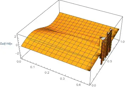
Plot3D[sol[x, t], {x, t} ∈ Rectangle @@ Transpose @ sol["Domain"]]