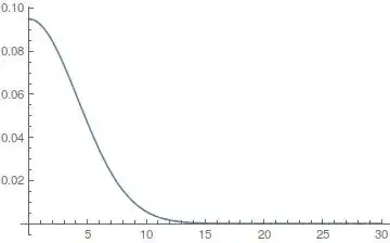
I need to N[Integrate] a function Cos[alpha*x]*f(x) between x=0 and 30 at increasing alpha-values. Here f(x) is an interpolated function derived from a set of 120 equally-spaced points belonging to the Gaussian 0.095*Exp[-x^2/35.28] between x=0 and 30. An example for alpha=2 is given below:
curve = Import["G1_theor_ZrH2.txt", {"Data", All, {1, 2}}]
intercurve = Interpolation[curve]
Plot[intercurve[x], {x, 0, 30}]
The interpolated function gets perfectly superimposed to the Gaussian in the above-mentioned range (and, in general, between x=-70 and 70).
Now, the problematic integrand is Cos[2*x]*intercurve[x], which is an oscillating Gaussian profile:
Plot[intercurve[x]*Cos[2*x], {x, 0, 30}, PlotRange -> Full]
Indeed, the exact integration of the exact curve over a non-finite range returns:
Integrate[0.095*Exp[-x^2/35.28]*Cos[2*x], {x, 0, Infinity}]
2.383*10^-16
If I try to perform an N[Integration] of the same exact curve over [0,50], I can find an accurate estimation if compared to the exact value:
N[Integrate[0.095*Exp[-x^2/35.28]*Cos[2*x], {x, 0, 50}], 20]
2.383*10^-16 + 5.90865*10^-47 I
If the integration range gets shrunk to [0,30] the evaluation turns out quite worse:
N[Integrate[0.095*Exp[-x^2/35.28]*Cos[2*x], {x, 0, 30}], 20]
1.18736*10^-13 + 0. I
When the same couple integrations is applied to the interpolated integrand, Mathematica returns:
N[Integrate[intercurve[x]*Cos[2*x], {x, 0, 50}], 20]
NIntegrate::slwcon: Numerical integration converging too slowly; suspect one of the following: singularity, value of the integration is 0, highly oscillatory integrand, or WorkingPrecision too small. >>
NIntegrate::eincr: The global error of the strategy GlobalAdaptive has increased more than 400 times. The global error is expected to decrease monotonically after a number of integrand evaluations. Suspect one of the following: the working precision is insufficient for the specified precision goal; the integrand is highly oscillatory or it is not a (piecewise) smooth function; or the true value of the integral is 0. Increasing the value of the GlobalAdaptive option MaxErrorIncreases might lead to a convergent numerical integration. NIntegrate obtained -0.0000461585926263450153769201220002 and 1.79688309588571048164765344384`30.*^-18 for the integral and error estimates. >>
-0.0000461585926263450153769201220002
and
N[Integrate[intercurve[x]*Cos[2*x], {x, 0, 30}], 20]
NIntegrate::slwcon: Numerical integration converging too slowly; suspect one of the following: singularity, value of the integration is 0, highly oscillatory integrand, or WorkingPrecision too small.
NIntegrate::eincr: The global error of the strategy GlobalAdaptive has increased more than 400 times. The global error is expected to decrease monotonically after a number of integrand evaluations. Suspect one of the following: the working precision is insufficient for the specified precision goal; the integrand is highly oscillatory or it is not a (piecewise) smooth function; or the true value of the integral is 0. Increasing the value of the GlobalAdaptive option MaxErrorIncreases might lead to a convergent numerical integration. NIntegrate obtained -0.0000461616042074379102542229207380 and 1.7968766559320907492916850148`30.*^-18 for the integral and error estimates. >>
-0.0000461616042074379102542229207380
Trying to enlarge MaxErrorIncrease as suggested has no healing effect:
NIntegrate[intercurve[x]*Cos[2*x], {x, 0, 30}, WorkingPrecision -> 20,
AccuracyGoal -> Infinity,
Method -> {"GlobalAdaptive", "MaxErrorIncreases" -> 10000}]
-0.000046161604207438302512
I also tried to both partition the integral of the interpolated function into a sum of integrations between pairs of zeroes and artificially 'inflate' the integrand by a suitable constant factor to be removed later, but niet.
As expected, things go fine at lower values of alpha (alpha<0.7) for both the exact and the interpolated integrand, due to the decrease in number of oscillations and the dramatic increase in global subtended area, which makes the contribution from the removed Gaussian tails non-significant.
However, my question is: why the same N[Integration] of Cos[2*x]*intercurve[x] and Cos[2*x]*0.095*Exp[-x^2/35.28] returns values that different, despite the two functions being visually identical over the same integration range?


WorkingPrecision– Lukas May 27 '16 at 10:31WorkingPrecisionmake results show a larger number of digits, but does not improve their accuracy. – Alexandra May 27 '16 at 12:43WorkingPrecision->100forNIntegrate– Lukas May 27 '16 at 13:05curvature– Lukas May 27 '16 at 13:06WorkingPrecision=100 makes Mathematica fail to converge near {x} = {1.25.....} and return the usual result (-0.00004616...). – Alexandra May 27 '16 at 13:48Integrateexpressions are returning machine precision values (indeed you have machine precision values in the input expression). Wrapping them inN[..,20]isn't doing anything. – george2079 May 27 '16 at 14:07Method -> "InterpolationPointsSubdivision"to yourNIntegrate[]involving the interpolated function that you have? – J. M.'s missing motivation May 27 '16 at 15:57MaxSubregionsoption ofInterpolationPointsSubdivisionto the number of intervals created by the interpolation points could produce more accurate results, but I don't know where to recover this number. – Alexandra May 27 '16 at 16:48