Factorisation diagrams

Question

Here is a way to visualize the factorisation of natural numbers. How do we get this or a similar kind of output using Mathematica?

See the list of images generated for number from 1 to 36:

factorisation diagrams for 1 to 36

This reminds me of Richard Schwartz's book You Can Count on Monsters. — Michael Wijaya, Oct 06 '12 at 19:31

Andrew Moylan · Answer 1 · 2012-10-06T18:37:01.593

Here is a recursive method using Outer:

FactorPoints[{1}] := {{0, 0}}

FactorPoints[{n_}] := 
 3/2 Csc[Pi/n] Through[{Cos, Sin}[# (2 Pi)/n]] & /@ Range[n]

FactorPoints[{n_, rest__}] := 
 Flatten[Outer[Plus, 9/4 Csc[Pi/n] FactorPoints[{rest}], 
   FactorPoints[{n}], 1], 1]

FactorPlot[n_] := 
 Graphics[Disk /@ 
   FactorPoints[Sort[Flatten[ConstantArray @@@ FactorInteger[n]]]]]

E.g. FactorPlot[30]:

Factor plot of 30 == 5 * 3 * 2

And Grid[Partition[Table[Show[FactorPlot[n], ImageSize -> 60], {n, 36}], 6], Frame -> All]:

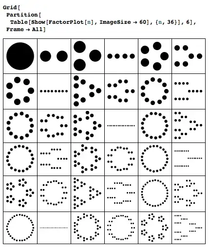
First attempt at replicating factor plot table

Some manual tweaking will be required to get the same layout as in your example above. In particular, the special case FactorPoints[{2, 2}] should be implemented to get the nice square shape that has been chosen in your original example:

FactorPoints[{2, 2, rest___}] := FactorPoints[{4, rest}]

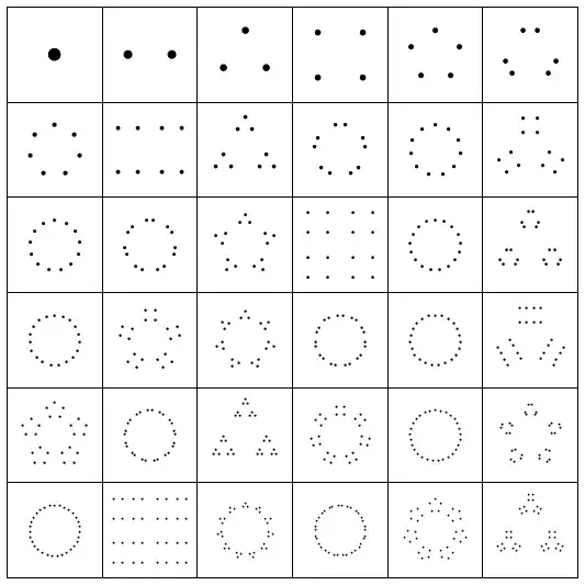
Then you get very close, except for some choices about orientation of each piece:

Better attempt at factor plot table

+1 for ConstantArray @@@ -- among other things. ;-) – Mr.Wizard Oct 07 '12 at 13:12 — Mr.Wizard, Oct 07 '12 at 13:12

faleichik · Answer 2 · 2012-10-10T17:26:35.617

Let me introduce the following animated approach: enter image description here

As you can see, I've slightly changed the way of diagram generation. The main differences are the following.

1. Now the diagrams are more symmetric. This is due to proper rotation after each sudivision.

2. As the main principle is to use factors in decreasing order, I consider 4 as a separate factor and place it before 3.

It is also should be noted that the total area of dots in each diagram is constant.

factorMovie[n_, fpm_, opts___] := 
  Module[{k, r0, r1, len, disksat, splitpts, pts, ns, prange, frames, 
    ptsat, line},
   line[t_] := t^2 (-1 + 2 t (7 + 2 t (-5 + 2 t)));
   disksat[t_] := Disk[# , r0 (1 - t) + r1 t] & @@@ ptsat[line@t];
   ptsat[t_] := {#1 + t len {Sin@#2, Cos@#2}, #2} & @@@ pts;

   splitpts[nn_] := Block[{},
     r0 = r1;
     r1 = r0/Sqrt[nn];
     pts = 
      Sequence @@ Table[{#1, #2 + (2 \[Pi])/nn i}, {i, 0, nn - 1}] & @@@
        ptsat[1];
     len *= Sin[\[Pi]/k]/(3 Sin[\[Pi]/nn]); k = nn;
     ];
   r0 = 1.5;
   len = 5;
   prange = 8;
   ns = Flatten[
      ReplaceRepeated[
       Table[#1, {#2}] & @@@ 
        FactorInteger[n], {a___, 2, 2, b___} :> {a, 4, b}]]~Sort~
     Greater;
   k = ns[[1]];
   r1 = r0/Sqrt[k];
   AppendTo[ns, ns[[-1]]];
   pts = Table[{{0, 0}, (2 \[Pi])/k i}, {i, 0, k - 1}] // N;
   frames = {};
   Do[
    frames = 
     frames~Join~
      Table[Graphics[disksat[t], PlotRange -> prange, opts], {t, 0, 1,
         1/fpm}];
    splitpts[m],
    {m, Rest@ns}
    ];
   frames
   ];

movies = Table[factorMovie[n, 10, ImageSize -> 80], {n, 2, 36}];
mlen = Max[Length /@ movies];
PrependTo[movies, Table[movies[[1, 1]], {mlen}]];
ms = If[(l = Length[#]) < mlen,
     Join[#, Table[#[[-1]], {mlen - l}]], #] & /@ movies;
frames = GraphicsGrid[Partition[#, 6], Frame -> All] & /@ 
   Transpose[ms];
ListAnimate[frames~Join~Reverse@frames, 
 AnimationDirection -> ForwardBackward]

And finally one more factoring movie for 420: enter image description here

n = 7 5 4 3
movie = factorMovie[n, 25, ImageSize -> 640];
frames = Join[Table[First@movie, {5}], movie, Table[Last@movie, {5}]];
ListAnimate[frames, 25, AnimationDirection -> ForwardBackward]

UPDATE

I've modified the rules of diagram generation regarding Andrew's comment below. Now the factoring is mathematically strict in a sense that 4 is not considered prime like above.

enter image description here

Here is the animatied version.

I've also cleaned the code but still it needs some tweaking which I don't have time for.

factorMovie[n_, fpm_, opts___] := 
  Module[{k, r0, r1, len, disksat, splitpts, pts, ns, prange, frames, 
    ptsat, line, s},
   line[t_] := t^2 (-1 + 2 t (7 + 2 t (-5 + 2 t)));
   disksat[t_] := Disk[#, r0 (1 - t) + r1 t] & @@@ ptsat[line@t];
   ptsat[t_] := {#1 + t len {Sin@#2, Cos@#2}, #2} & @@@ pts;
   splitpts[nn_] := Block[{}, r0 = r1;
     r1 = r0/Sqrt[nn];
     pts = 
      Sequence @@ 
         Table[{#1, #2 + \[Pi] (1 + 2 i + nn)/nn }, {i, nn}] & @@@ 
       ptsat[1];
     len *= 
      If[k == nn == 2, (4/9)^(s = 1 - s), 
       Sin[\[Pi]/k]/(3 Sin[\[Pi]/nn])];
     k = nn;
     ];
   r0 = r1 = 1;

   prange = 7;
   ns = Flatten[Table[#1, {#2}] & @@@ FactorInteger[n]]~Sort~Greater;
   k = First@ns;
   {len, s} = If[k == 2, {8, 0}, {12, 1}];
   pts = {{{0, -len}, 0}};
   frames = {};
   Do[
    splitpts[m];
    frames = 
     frames~Join~
      Table[Graphics[disksat[t], PlotRange -> prange, opts], {t, 0, 1,
         1/fpm}]
    , {m, ns}];
   frames
   ];

movies = Table[factorMovie[n, 8, ImageSize -> 80], {n, 2, 36}];
mlen = Max[Length /@ movies];
PrependTo[movies, Table[movies[[1, 1]], {mlen}]];
ms = If[(l = Length[#]) < mlen, 
     Join[#, Table[#[[-1]], {mlen - l}]], #] & /@ movies;
frames = GraphicsGrid[Partition[#, 6], Frame -> All] & /@ 
   Transpose[ms];
ListAnimate[frames, AnimationDirection -> ForwardBackward]

And finally this is the modified version of factoring 420.

Excellent work. These are beautiful! I agree, a rotation is the proper solution to get diagram symmetry. Question: Do you really need the special case for n=4 when you have the rotation? — Andrew Moylan, Oct 10 '12 at 01:57
@Andrew, thank you, this is a good idea, though it will require to adjust spacing factor for n=2 to get nice pictures. I will update the answer soon. — faleichik, Oct 10 '12 at 12:47
Amazing! However, you have some spacing issues with lots of 11 and 13 factors that end up with overlapping rings. — s0rce, Oct 10 '12 at 17:58
Yep, this is the one of issues: need to adjust the rule for subsequent indentations... — faleichik, Oct 10 '12 at 18:06
Your final animation http://i.stack.imgur.com/5d9Ld.gif is mesmerizing! — Andrew Moylan, Oct 11 '12 at 20:58
You might enjoy seeing this, which is nearly as good as yours! — cormullion, Nov 05 '12 at 17:09

score 21 · Answer 3 · answered Oct 06 '12 at 18:44

Here's my modest attempt:

shiftMe[g_, 1] := g

shiftMe[g_, {2, tag_Integer?Positive}] := If[OddQ[tag],
  Translate[Scale[g, 1/2], #] & /@ {{0, 1}, {0, -1}}, 
  Translate[Scale[g, 1/2], #] & /@ {{1/2, 0}, {-1/2, 0}}]

shiftMe[g_, k_?PrimeQ] := Translate[Scale[g, 1/k], 
     Through[{Cos, Sin}[2 π #/k - π/(2 k)]]] & /@ Range[0, k - 1] /; k > 2

factorizationDiagram[n_Integer?Positive] := Graphics[Fold[shiftMe,
   {Disk[{0, 0}, 1]}, 
   MapIndexed[If[#1 == 2, Prepend[#2, 2], #1] &, 
    Flatten[ConstantArray @@@ FactorInteger[n]]]]]

Map[factorizationDiagram, Partition[Range[36], 6], {2}] // GraphicsGrid

factorization diagrams

score 13 · Answer 4 · edited Apr 23 '14 at 20:42

Szabolcs found a page that does animated transitions between the diagrams in JavaScript here. Here's an iterative implementation of the diagrams and some basic animated transitions between them.

DynamicModule[{shapes, t, n, next, keyframes}, 
 shapes[i_] := 
  Thread@{Table[
     ColorData["BlueGreenYellow"]@Rescale[a, {1, i}], {a, i}], 
    Disk /@ First@
      Fold[Module[{pts = #[[1]], r = #[[2]], 
          n = #2}, {Join @@ 
           Table[# + n r Through@{Cos, Sin}[a 2 Pi/n + Pi/2] & /@ 
             RotationTransform[a 2 Pi/n + If[n == 2, Pi/2, 0]]@
              pts, {a, n}], n r}] &, {{{0., 0.}}, 1}, 
       Join @@ ConstantArray @@@ FactorInteger@i]};
 t = 1;
 n = 1;
 next[] := 
  keyframes = 
   Thread[{Prepend[#, #[[1]]], #2} & @@ (shapes /@ {n, n + 1})];
 next[];
 Dynamic[If[(t += .02) >= n + 1, n++; next[]];
  Graphics[{Blend[{#[[1]], #2[[1]]}, t - n], 
      Disk[#[[2, 1]] + (t - n) (#2[[2, 1]] - #[[2, 1]])]} & @@@ 
    keyframes, PlotRange -> t*{{-2, 2}, {-2, 2}}, AspectRatio -> 1, 
   ImageSize -> 300]]]

enter image description here

Again, great! And thanks for refreshing this Q&A, I've not seen it yet. — Kuba, Apr 23 '14 at 20:11
Thanks! I'll update it with halirutan's PlotRange improvement. — Michael Hale, Apr 23 '14 at 20:39

score 9 · Answer 5 · answered Oct 07 '12 at 15:28

This is Andrew's method with a few tweaks of my own. The addition of the adjustment argument should make other customization a bit easier.

f[{1}] = {{0, 0}};

f[{2}] = {{0, -9}, {0, 9}}/8;

f[{2, 2, rest___}] := f[{4, rest}, RotationMatrix[π/4]]

f[{n_}, adj___] := 
  Array[3/2 Csc[π/n] {Cos@#, Sin@#} &[# 2 π/n + π/2] &, n].adj

f[{n_, rest__}, adj___] := 
  Tuples@{9/4 Csc[π/n] f[{rest}], f[{n}].adj} ~Total~ {2}

FactorPlot[n_, opts___] := 
  Graphics[Disk /@ f[Join @@ ConstantArray @@@ FactorInteger @ n], opts]

Grid[Array[FactorPlot[#, ImageSize -> {90}] &, 36] ~Partition~ 6, Frame -> All]

Mathematica graphics

Factorisation diagrams

5 Answers5

Linked