Numerically parameterize portion of $F[x,y]==0$

Question

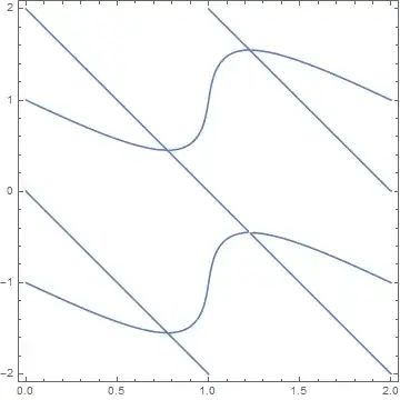
I have a relatively complicated function of two variables F[x,y] whose zero locus contains a number of intersecting paths in the $x,y$-plane. A problem I've been struggling with for a great while now is numerically parameterizing precisely one of these paths. Meaning, I want to collect a large number of tuples $(x,y)$ precisely lying on one of these paths. I include my code with all the preamble:

M = 1;
tau = (0.5) + (0.4)*I;
w1 = Pi/2;
w2 = Pi*(tau)/2;
inv = WeierstrassInvariants[{w1, w2}];
E2[t_] = 1 - 24*Sum[(n*Exp[2*Pi*I*(t)*n])/(1 - Exp[2*Pi*I*(t)*n]), {n, 1, 300}];
z[u_] = (I*M/2)*(WeierstrassZeta[u, inv] - ((1/3)*N[E2[tau], 50]*(u)));
WP[x_, y_] = WeierstrassP[w1*x + w2*y, inv];
L = -(1/3)*N[E2[tau], 50];
f[x_, y_] = Re[WP[x, y] - L];
g[x_, y_] = Im[WP[x, y] - L];
ContourPlot[{f[x, y] == 0, g[x, y] == 0}, {x, 0, 2}, {y, -2, 2}]
V1 = Quiet[FindRoot[{f[x, y] == 0, g[x, y] == 0}, {x, 0.8}, {y, 0.5}, WorkingPrecision -> 50]];
V2 = Quiet[FindRoot[{f[x, y] == 0, g[x, y] == 0}, {x, 1.2}, {y, 1.5}, WorkingPrecision -> 50]];
V3 = Quiet[FindRoot[{f[x, y] == 0, g[x, y] == 0}, {x, 0.8}, {y, -1.5}, WorkingPrecision -> 50]];
V4 = Quiet[FindRoot[{f[x, y] == 0, g[x, y] == 0}, {x, 1.2}, {y, -0.5}, WorkingPrecision -> 50]];
A1 = x /. V1;
B1 = y /. V1;
A2 = x /. V2;
B2 = y /. V2;
A3 = x /. V3;
B3 = y /. V3;
A4 = x /. V4;
B4 = y /. V4;
Z1 = Quiet[N[z[w1*A1 + w2*B1], 50]];
Z2 = Quiet[N[z[w1*A2 + w2*B2], 50]];
Z3 = Quiet[N[z[w1*A3 + w2*B3], 50]];
Z4 = Quiet[N[z[w1*A4 + w2*B4], 50]];
m = (Im[Z1] - Im[Z2])/((Re[Z1] - Re[Z2]));
ListPlot[
  {{Re[Z1], Im[Z1]}, {Re[Z2], Im[Z2]}, {Re[Z3], Im[Z3]}, {Re[Z4], Im[Z4]}}, 
  PlotRange -> {{-5, 5}, {-5, 5}}
]

Zed[x_, y_] = z[w1*x + w2*y];

Quiet[ContourPlot[
        {Im[N[Zed[x, y]]] - (m*(Re[N[Zed[x, y]]] - Re[(M/2)]) - Im[M/2]), 0}, 
        {x, 0, 2}, {y, -2, 2}, 
        MeshFunctions -> {#3 &}, MeshStyle -> {{Thick, Blue}}, Mesh -> {{0}}, 
  PlotStyle -> Directive[Orange, Opacity[0.1], Specularity[White, 30]], 
  PlotPoints -> 75, WorkingPrecision -> 50, ClippingStyle -> None
 ]
]

In this final contour plot there is a nice smooth path from $(0,1)$ to $(2,1)$. This is precisely the path I want to parameterize. Now, I want to have the parameter be something like length along the path; the coordinate $x$ is an insufficient parameter because this curve I'm interested in, in some cases, may cease to be a function of $x$.

I should emphasize, the function whose zero set I'm plotting at the end is

Im[N[Zed[x, y]]] - (m*(Re[N[Zed[x, y]]] - Re[(M/2)]) - Im[M/2])

I have a way of doing something like this in a very simple example which (almost) works. Since I know exactly my starting point $(0,1)$, I can compute the gradient of my function, take a tiny step along the tangent vector, and find a new point on the curve near the tip of the tangent vector. However, I'm worried this method will be wildly inefficient given that the function above contains fairly unwieldy modular functions and the like. Moreover, by method goes bad at points of intersection where the gradient of the function vanishes.

In principle, the method described above should work, but even on an incredibly trivial function I picked, it takes quite a lot of time and quickly breaks down near intersections. Can anyone think of an easier way of doing this numerical parametrization?