Plot Dirac Delta function

Question

I would like to know how to plot the Dirac Delta result of the Fourier transform of the following typical expression

tf = FourierTransform[(A Sin[ω1 t]) + (A2 Sin[ω2 t]), 
      t, ω, FourierParameters -> {1, -1}] // TraditionalForm

Answer 1

You can replace the delta functions with something you can plot, to get some sort of visualisation. E.g.

Block[{A = 1, A2 = 1.4, ω1 = 40, ω2 = -30, 
  DiracDelta = UnitTriangle}, Plot[Abs[tf], {ω, -50, 50}]]

Answer 2

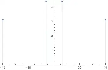
If your "typical expression" is a discrete sum of sine waves, then we might treat the delta function as the "unit" of the vertical axis and plot the magnitude of the coefficients.

Block[{A = 1, A2 = 1.4, ω1 = 40., ω2 = Sqrt@40.},
 freqs = Cases[tf, DiracDelta[f_] :> Root[f, 1], Infinity];
 DiscretePlot[
  Abs[tf] /. DiracDelta -> DiscreteDelta,
  {ω, freqs},
  AxesOrigin -> {0, 0}]
]

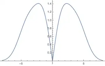
On the other hand, if there's a continuous spectrum, use Plot:

tf = FourierTransform[
   Exp[-t^2] (A Sin[ω1 t] + A2 Sin[ω2 t]), t, ω, 
   FourierParameters -> {1, -1}];
Block[{A = 1, A2 = 7/5, ω1 = 4, ω2 = Sqrt@2},
 Plot[Abs[tf], {ω, -8, 8}, WorkingPrecision -> 50]]

Answer 3

I think there are two different aspects here. First let add to sin signals, say, $\sin[(\omega+\Delta)t]$ and $\sin[(\omega-\Delta)t]$

Manipulate[ Plot[Sin[2 Pi (n + d) x] + Sin[2 Pi (n - d) x], {x, -5 Pi, 5 Pi}],
{n, 1, 10}, {d, 0, 1}]

As you can see the difference in frequency will give you beats. Now let say you want to create a Delta function like spectrum you have to add infinite number of Sin waves with proper weight. I choose here a gaussian weight. I choose Cos to make things symmetric.

Manipulate[Plot[Sum[Exp[-k^2 d^2] Cos[k x], {k, 0, 10, 0.1}], {x, -5 Pi, 5 Pi}, 
PlotRange -> All], {d, 0, 1}]

As you can see by controlling the gaussian width of distribution you can get a nice and sharp spike. For a true Dirac-Delta function you have to take the integration limit for k to infinity.