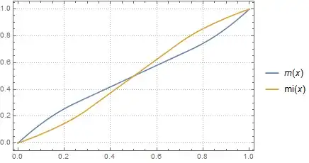
I have a B-spline function, which is a function that is defined as a weighted sum of BSplineBasis function:
p = 2;
knotvector := {0, 0, 0, 0.25, 0.5, 0.75, 1, 1, 1};
n := Length[knotvector] - p - 1;
controlvector := {0, .2, .4, .6, .8, 1};
m[\[Xi]_] := Sum[controlvector[[k]] * BSplineBasis[{p, knotvector}, k - 1, \[Xi]], {k, 1, n}];
It happens to have an inverse (I know this by how the weights are chosen). So, I want to calculate the inverse function:
mi := InverseFunction[m];
This works for most of the functions domain (0, 1). However, near 0, the derivative of the function is small, and Mathematica refuses to evaluate the function:
mi[.15] (* = 0.104715 *)
mi[0.05] (* returns unevaluated expression *)
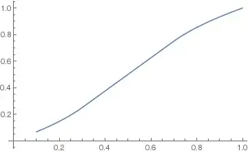
This can also be seen in a plot:
Plot[mi[x], {x, 0, 1}]
It seems the inverse can be calculated on approximately the interval (0.1, 1]. How can I get the inverse on the whole interval [0, 1]?
I have been struggling with this and related problems for several hours. I tried wrapping the expression with Evaluate[...] and N[...], to no avail. I have also tried defining an inverse in terms of FindRoot, which works fine for plotting, but gives me a lot of troubles when taking derivatives or using the inverse in a composite function (but I should ask a separate question about this).
In case someone gets different results: I have Mathematica 10.3.1.0 for Raspberry Pi.


psupposed to be? I'm guessing $2$ based on your choice of knot vector... – J. M.'s missing motivation Oct 15 '16 at 12:00mi = InverseFunction[Function[x, Evaluate[PiecewiseExpand[m[x], 0 < x < 1]]]];? – J. M.'s missing motivation Oct 15 '16 at 12:14