I'll show you a LaplaceTransform-based solution, mainly because it's the only approach I can think out that takes the finiteness condition into account properly.
First, by eliminating the intermediate variable $w$, the equation set becomes:
$$\frac{\partial (xu)}{\partial t} = \frac{\partial^2 (xu)}{\partial x^2}$$
$$\frac{\partial (xv)}{\partial t} = \frac{\partial^2 (xv)}{\partial x^2}$$
$$u(x,0)=1,\ v(x,0)=0$$
$$u(0,t)\ \text{is finite},\ v(g,t)=u(g,t),\ \frac{\partial u}{\partial x}\bigg| _{x= g} = \frac{\partial v}{\partial x}\bigg| _{x= g},\ \frac{\partial v}{\partial x}\bigg| _{x= g} =\frac{\partial v}{\partial t}\bigg| _{x= g}$$
Then we eliminate the derivatives of $t$ with LaplaceTransform and solve the obtained ODE set with DSolve:
eqn = {D[u[t, x] x, t] == D[u[t, x] x, x, x],
      D[v[t, x] x, t] == D[v[t, x] x, x, x]};
ic = {u[0, _]  -> 1, v[0, _] -> 0};
bc = {u[t, g] == v[t, g],
   D[u[t, x], x] == D[v[t, x], x] /. x -> g,
      D[v[t, x], x] == D[v[t, x], t] /. x -> g};

teqn = LaplaceTransform[{eqn, bc}, t, s] /. ic /.
  HoldPattern@LaplaceTransform[a_, __] :> a

tsol = {u[t, x], v[t, x]} /. First@DSolve[teqn, {u[t, x], v[t, x]}, x] // Simplify
(* tsol =
     {(E^(-Sqrt[s] (2 g + x)) (-E^(Sqrt[s] (g + 2 x)) (1 + g s + g^2 (-1 + Sqrt[s]) s) +
      E^(3 g Sqrt[s]) (1 + g (-2 Sqrt[s] + s) + g^2 (s - s^(3/2))) +
      2 E^(Sqrt[s] (2 g + x)) Sqrt[s] (1 + g (-Sqrt[s] + s)) x +
      2 E^(2 g Sqrt[s]) s^(3/2) (1 + g (-Sqrt[s] + s)) C[3] -
      2 E^(2 Sqrt[s] x) s^(3/2) (1 + g (Sqrt[s] + s)) C[3]))/(2 s^(
    3/2) (1 + g (-Sqrt[s] + s)) x), (
 E^(-Sqrt[s] (2 g + x)) (E^(2 g Sqrt[s]) (1 + g (-Sqrt[s] + s)) -
    E^(2 Sqrt[s] x) (1 + g (Sqrt[s] + s))) C[3])/((1 + g (-Sqrt[s] + s)) x)}; *)
Remark
HoldPattern@LaplaceTransform[a_, __] :> a is needed because DSolve
can't handle expression containing LaplaceTransform properly. Just
remember u[t, x] etc. in teqn actually represents
LaplaceTransform[u[t, x], t, s].
As expected, tsol still contains a constant C[3] because we haven't impose the finiteness condition for $u(0,t)$, and this is the first obstacle.
How to overcome?
Let's observe the form of tsol. We'll easily find that it involves 1/x term. Apparently it should not exist in a solution that is bounded at $x=0$, so the coefficient of it should be 0 at $x=0$. By Collecting the 1/x term:
Collect[tsol, 1/x, FullSimplify]
(* {1/s + (E^(-Sqrt[s] (2 g + x)) (-E^(Sqrt[s] (g + 2 x)) (1 + g (1 + g (-1 + Sqrt[s]))s)-
        E^(3 g Sqrt[s]) (-1 + g Sqrt[s]) (1 + g (-Sqrt[s] + s)) +
       2 E^(2 g Sqrt[s]) s^(3/2) (1 + g (-Sqrt[s] + s)) C[3] -
       2 E^(2 Sqrt[s] x) s^(3/2) (1 + g (Sqrt[s] + s)) C[3]))/(2 s^(
     3/2) (1 + g (-Sqrt[s] + s)) x), (
 E^(-Sqrt[s] (2 g + x)) (E^(2 g Sqrt[s]) (1 + g (-Sqrt[s] + s)) -
    E^(2 Sqrt[s] x) (1 + g (Sqrt[s] + s))) C[3])/((1 + g (-Sqrt[s] + s)) x)} *)
The coefficient becomes clear, so does the value of C[3]:
solC = First@
  Solve[0 == (E^(-Sqrt[
         s] (2 g + x)) (-E^(Sqrt[s] (g + 2 x)) (1 + g (1 + g (-1 + Sqrt[s])) s) -
         E^(3 g Sqrt[s]) (-1 + g Sqrt[s]) (1 + g (-Sqrt[s] + s)) +
         2 E^(2 g Sqrt[s]) s^(3/2) (1 + g (-Sqrt[s] + s)) C[3] -
         2 E^(2 Sqrt[s] x) s^(3/2) (1 + g (Sqrt[s] + s)) C[3])) /. x -> 0, C[3]]
Substitute C[3] to tsol, we obtain the transformed solution of $u$ and $v$:
{utfunc[s_, x_], vtfunc[s_, x_]} = Simplify[tsol /. solC] /. g -> 11/10
The final step is to transform the solution back, but a naive utilization of InverseLaplaceTransform fails, so we encounter another obstacle and need to overcome it with numeric inverse Laplace transform. Here I'll use the FT function in this package:
ufuncgenerator[x_] :=
 ufuncgenerator[x] = Module[{t}, Compile[#, #2] &[t, FT[utfunc[#, x] &, t]]]
vfuncgenerator[x_] :=
 vfuncgenerator[x] = Module[{t}, Compile[#, #2] &[t, FT[vtfunc[#, x] &, t]]]

ufunc = Function[{t, x}, ufuncgenerator[x][t]]
vfunc = Function[{t, x}, vfuncgenerator[x][t]]
Remark
A somewhat advanced function Compile is used for speeding up. Here
you can simply understand it as a fast Function. If you're not that
familiar with Mathematica, I don't recommend you to look into it.
Now $u$ can be easily calculated:
Plot3D[ufunc[t, x], {t, 0, 1}, {x, -1, 11/10}]

However, $v$ seems to be a little troublesome when $t$ is small:
Plot3D[vfunc[t, x], {t, 0, 1}, {x, -1, 11/10}]

But wait, isn't the solution of $v$ a bit too similar to $u$? Indeed, 2nd and 3rd b.c. indicate that the b.c. for $u$ and $v$ is the same, though their i.c.s are different, it's not strange that an inconsistent i.c. is largely (or even totally) ignored in the final solution. Can they be the same? To examine this guess, let's make the inverse transform with NIntegrate, thus we encountered the 3rd obstacle because NIntegrate can't calculate Bromwich integral properly if we naively choose something like $(1-i\infty)\to(1+i\infty)$ as the integrating path. Based on the experience in this post, I choose the path $(-\infty-i\infty)\to(-\infty-i\epsilon)\to(\epsilon-i\epsilon)\to(\epsilon+i\epsilon)\to(-\infty+i\epsilon)\to(-\infty+i\infty)$ where $\epsilon$ is a positive number:
nil[f_, t_, eps_: 10^-6, prec_: MachinePrecision] :=
 2 Re[1/(2 π I) NIntegrate[f@s Exp[s t], {s, -Infinity - eps I, eps - eps I},
      MaxRecursion -> 100, WorkingPrecision -> prec]] +
  1/(2 π I) NIntegrate[f@s Exp[s t], {s, eps - eps I, eps + eps I},
    MaxRecursion -> 100, WorkingPrecision -> prec]

Plot3D[nil[(vtfunc[#1, x] &), t] // Re, {t, 0, 1}, {x, -1, 11/10},
  PlotRange -> All] // AbsoluteTiming
(* 1075.172149 <- a bit time consuming *)
Remark
// Re is added to remove the small imaginary part produced by
numeric error.

OK, though the error near $t=0$ is still a little significant, it's much better.
Now we can slice at a small $t$ and compare:
dat = With[{t = 10^-3},
    ParallelTable[{ufunc[t, x], nil[(vtfunc[#1, x] &), t] // Re} // Quiet, {x, -1, 11/10,
       21/10/100}, DistributedContexts -> All]]; // AbsoluteTiming

(* {36.362744, Null} *)

ListLinePlot[dat // Transpose, PlotRange -> {0, 2},
 PlotStyle -> {{Thin}, {Dashed, Thick}}]
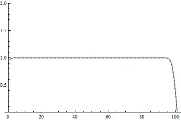
Given that the solution matches well even at a small $t$ and the b.c. of $u$ and $v$ is the same, I think it's safe to say $u$ and $v$ is (at least almost) identical in this case.