No result from DSolve

Question

I don't get any answer when I evaluate the following expression:

DSolve[{x'[t] == -0.5*y[t] + 1 + 3*(e^(-2*t)), 
        y'[t] == 2*x[t] - y[t] - 4 - 4* (e^(-t)), 
        y[0] == 0, x[0] == 0}, {x[t], y[t]} , t]

Did I go wrong somewhere?

I tried solving this equation set with Laplace as well, but I didn't get any answer from that either.

2

Is it e, or E ? – Dr. belisarius Oct 17 '12 at 17:28

Dr. belisarius · Accepted Answer · 2012-10-17T17:59:32.680

6

Try replacing the .5by 1/2 and the e by E. Also, the asterisks aren't needed in Mathematica.

s = DSolve[
 {x'[t] == -1/2 y[t] + 1 + 3 E^(-2 t),
  y'[t] == 2 x[t] - y[t] - 4 - 4 E^(-t),
  y[0]  == 0, 
  x[0]  == 0}, {x[t], y[t]}, t]

ParametricPlot[{x[t], y[t]} /. s, {t, 0, 10}, AxesOrigin -> {0, 0}]

Mathematica graphics

edited Oct 17 '12 at 17:59

answered Oct 17 '12 at 17:29

Dr. belisarius

115,881
13
203
453

and //FullSimplify ;) – Vitaliy Kaurov Oct 17 '12 at 17:32
@VitaliyKaurov Tried that, but the result isn't compact enough to look nice here. So I kept it like that. – Dr. belisarius Oct 17 '12 at 17:34
1

That was more a tip for @DSaad than an edit suggestion :) – Vitaliy Kaurov Oct 17 '12 at 17:36

Artes · Answer 2 · 2012-10-18T11:14:32.493

Two problems here are e instead of E and 0.5 instead of 1/2. For a larger system it would be more reasonable to use Rationalize instead of substituting all numbers by hand. To get a wider class of solutions we could define a function being a solution of the system of differential equations, where the initial values are parametrized by x0:

ds[x0_] = Simplify @ DSolve[ Rationalize @ {x'[t] == -0.5*y[t] + 1 + 3*(E^(-2*t)),
                                            y'[t] == 2*x[t] - y[t] - 4 - 4*(E^(-t)), 
                                            y[0] == 0, 
                                            x[0] == x0},     {x[t], y[t]}, t]

enter image description here

originally x0 == 0, i.e.

ds[0]

enter image description here

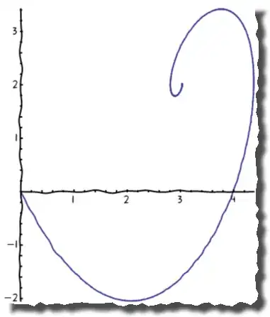
To plot the wider class of solutions we could use ParametricPlot as in belisarius answer with Show emphasizing ds[0] solution as a red thick curve :

Show[
      ParametricPlot[{x[t], y[t]} /. Table[ds[x0], {x0, -2, 4, 0.2}],
                                                   {t, -1, 10}, Evaluated -> True], 
      ParametricPlot[{x[t], y[t]} /. ds[0], {t, -1, 10}, 
                                             PlotStyle -> {Darker@Red, Thickness[0.007]}],
      AxesOrigin -> {0, 0}, PlotRange -> {{-1, 6}, {-4, 5}}]

enter image description here

No result from DSolve

2 Answers2

Linked

Related