Singularities using VectorPlot

Question

I am trying to plot a vector function of a fluid flow given by

$\vec{V} = (\frac{-\cos(\theta)}{r^2},-\frac{\sin(\theta)}{r^2})$

I am trying to plot it in Mathematica using the command below, I converted to Cartesian coordinates by the way. But this does not run in Mathematica. Without the Exclusions option, I only get one arrow at the origin. Can you help me with this plot?

VectorPlot[
      {-(x/(x^2 + y^2)^(3/2)), -(y/(x^2 + y^2)^(3/2))}, 
      {x, -1, 1}, {y, -1, 1}, 
      Exclusions -> {(x^2 + y^2)^(3/2) == 0} 
 ]

Welcome to Mathematica.SE! I suggest the following: 1) As you receive help, try to give it too, by answering questions in your area of expertise. 2) Read the FAQs! 3) When you see good Q&A, vote them up by clicking the gray triangles, because the credibility of the system is based on the reputation gained by users sharing their knowledge. ALSO, remember to accept the answer, if any, that solves your problem, by clicking the checkmark sign. — Vitaliy Kaurov, Oct 21 '12 at 07:59
Exclusions is not an option of VectorPlot. If you include it you only get an error message and no plot at all. — Sjoerd C. de Vries, Oct 21 '12 at 13:26
This is basically the same as Visualizing a Complex Vector Field near Poles - I'm sure you can adapt one of the answers from that question. — Jens, Oct 21 '12 at 17:04

Vitaliy Kaurov · Answer 1 · 2012-10-22T00:12:45.630

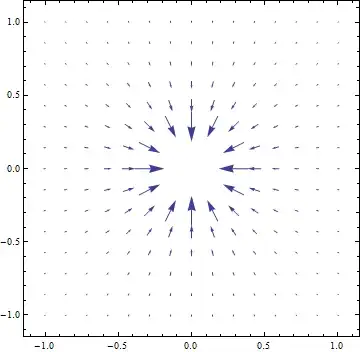
You can make use of option VectorScale - see the "More Information" section, and some singular examples at the end. Setting None will cause all the vectors to have the same length. Or you can improvise with a custom function to make the best view of the arrows (#5 the fifth argument is vector's norm):

VectorPlot[{-(x/(x^2 + y^2)^(3/2)), -(y/(x^2 + y^2)^(3/2))}, {x, -1, 1}, {y, -1, 1},
VectorScale -> {Automatic, Automatic, #}] & /@ {None, Function[If[#5 > 50, None, #5^.3]]}

enter image description here

You can also use StreamPlot

StreamPlot[{-(x/(x^2 + y^2)^(3/2)), -(y/(x^2 + y^2)^(3/2))}, {x, -1, 1}, {y, -1, 1}]

enter image description here

----- Edit: adding potential - as requested in the comments ----------

In your case potential is easily computed as integral over corresponding coordinates. Note automating clipping in the plot range. Here is the result with VectorPlot:

Show[ContourPlot[1/Sqrt[x^2 + y^2], {x, -1, 1}, {y, -1, 1}, 
  ContourStyle -> Directive[Red, Dashed], ColorFunction -> "Rainbow", Contours -> 20],
 VectorPlot[{-(x/(x^2 + y^2)^(3/2)), -(y/(x^2 + y^2)^(3/2))}, {x, -1, 1}, {y, -1, 1}, 
  VectorScale -> {Automatic, Automatic, 
         Function[If[#5 > 50, None, #5^.3]]}, VectorStyle -> Black]]

enter image description here

and StreamPlot styled a bit differently

Show[ContourPlot[1/Sqrt[x^2 + y^2], {x, -1, 1}, {y, -1, 1}, 
  ContourStyle -> Directive[Red, Dashed], ColorFunction -> "GrayTones"],
 StreamPlot[{-(x/(x^2 + y^2)^(3/2)), -(y/(x^2 + y^2)^(3/2))}, {x, -1, 1}, {y, -1, 1}, 
     StreamStyle -> White]]

enter image description here

Thanks for this! This is for a fluid flow by the way. Is there an easy way to quickly draw the streamfunction and potential function (prependicular to each other) on the same graph? — l3win, Oct 21 '12 at 17:14

Sjoerd C. de Vries · Answer 2 · 2012-10-21T18:53:36.233

7

Exclusions is not an option of VectorPlot. As an alternative, you could use Boole to exclude part of the plot:

VectorPlot[
    Boole[x^2 + y^2 > 0.08] {-(x/(x^2 + y^2)^(3/2)), -(y/(x^2 + y^2)^(3/2))}, 
    {x, -1, 1}, {y, -1, 1}
]

Mathematica graphics

Combining this with the potential:

Show[
 DensityPlot[1/Sqrt[x^2 + y^2], {x, -1, 1}, {y, -1, 1}, 
  ColorFunction -> "SolarColors"],
 VectorPlot[
  Boole[x^2 + y^2 > 
     0.1] {-(x/(x^2 + y^2)^(3/2)), -(y/(x^2 + y^2)^(3/2))}, {x, -1, 
   1}, {y, -1, 1}]
 ]

Mathematica graphics

edited Oct 21 '12 at 18:53

answered Oct 21 '12 at 13:30

Sjoerd C. de Vries

65,815
14
188
323

Thank you all for the messages, you have been very helpful. I have one more question. The above was my vector field. Is there any way I can plot the potential function of my vector field? $\vec{V} = \nabla(f)$ How can I plot f? – l3win Oct 21 '12 at 18:34
I still get a different scalar potential. This seems to me like a single sink, I get a dipole... Thanks for all the replies though – l3win Oct 22 '12 at 16:53
@I3win have you calculated the gradient of 1/Sqrt[x^2+y^2]? I got the vector field in your code example. The vector plot is consistent with tat, not with te field of a dipole. – Sjoerd C. de Vries Oct 22 '12 at 19:09

Singularities using VectorPlot

2 Answers2

Linked

Related