12

Context

In a previous post, I learned how to produce these kind of plots, which are of interest in astrophysics and geophysics.

Mathematica graphics Mathematica graphics

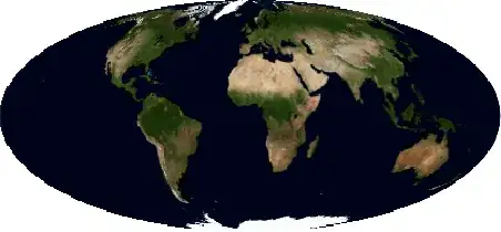
I am now interested in combining them.

Attempt

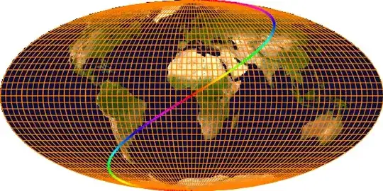
For this purpose, @belisarius suggested using the command

ImageCompose[mollwide, grid /. Line[a__] :> {White, Line[a]}]

which produces this (note the incorrect scaling)

Mathematica graphics

As an other example (to make this question self contained) let us look at StreamPlot

 gr = StreamPlot[{-1 - x^2 + y, 1 + x - y^2}, {x, -Pi, Pi}, {y, -Pi/2,
 Pi/2}, AspectRatio -> 1/2, Frame -> False];
 cart[{lambda_, phi_}] :=  With[{theta = fc[phi]}, {2 /Pi*lambda Cos[theta],   Sin[theta]}];
 fc[phi_] := Block[{theta}, If[Abs[phi] == Pi/2, phi,  theta /. 
 FindRoot[2 theta + Sin[2 theta] == Pi Sin[phi], {theta, phi}]]];

 gr2 = gr /. Arrow[pts_] :> Arrow[(cart /@ pts)] /. 
 Point[pts_] :> Point[cart[ pts]] // 
 Show[#, PlotRange -> {{-2, 2}, {-1, 1}}] &;

 i = Import["http://tpfto.files.wordpress.com/2012/02/firemap.png"];
 invmollweide[{x_, y_}] := With[{theta = ArcSin[y]}, {Pi (x)/(2 Cos[theta]), 
 ArcSin[(2 theta + Sin[2 theta])/Pi]}];
 moll = ImageTransformation[i, invmollweide, DataRange -> {{-Pi, Pi}, {-Pi/2, Pi/2}}, 
 PlotRange -> {{-2, 2}, {-1, 1}}, Padding -> White];

 ImageCompose[ImageResize[moll, 1200], 
 gr2 /. Arrow[a__] :> {AbsoluteThickness[3], White, Arrow[a]}]

Mathematica graphics

Question

  1. How can I make sure the image size match?
  2. How can I combine them so that the grid remains a vector image rather than a raster?
chris
  • 22,860
  • 5
  • 60
  • 149
  • Surely ImageResize[] can be appropriately applied... – J. M.'s missing motivation Oct 21 '12 at 13:42
  • @J.M. It sort of helps in fact: ImageCompose[ImageResize[moll, 800], grid /. Line[a__] :> {AbsoluteThickness[2], White, Line[a]}] produces this mollweide with grid which is better in terms of resolution, but the global scaling remains the same. – chris Oct 21 '12 at 13:47
  • 2
    Do you use PlotRangePadding -> 0 in your plots? That's usually one way of removing unwanted margins in plots... – cormullion Oct 21 '12 at 14:12
  • @cormullion Yes! gr2 = gr /. Arrow[pts_] :> Arrow[(cart /@ pts)] /. Point[pts_] :> Point[cart[ pts]] // Show[#, PlotRange -> {{-2, 2}, {-1, 1}},PlotRangePadding -> 0]] &; does the trick; please post your answer? – chris Oct 21 '12 at 14:17
  • @chris, will post what I had, for what it's worth – cormullion Oct 21 '12 at 14:34

2 Answers2

14

You can use Inset to place the image inside a vector graphics. Inset has various parameters to set the size and position of the image places. To test it you could use a scaled version of an image and overlay it with a grid. You see the lines match exactly:

img = ImageResize[ExampleData[{"TestImage", "Lena"}], {100, 100}];
Graphics[{Inset[img, {0, 0}, {0, 0}, {100, 100}], Line[#], 
    Line[Transpose[#]]}, PlotRange -> {{-1, 101}, {-1, 101}}] &@
 Table[{i, j}, {i, 0, 100, 5}, {j, 0, 100, 5}]

Mathematica graphics

Earth

Using this in your application, you would only have to copy all the code snips:

cart[{lambda_, phi_}] := 
 With[{theta = fc[phi]}, {2/Pi*lambda Cos[theta], Sin[theta]}]
fc[phi_] := 
  Block[{theta}, 
   If[Abs[phi] == Pi/2, phi, 
    theta /. 
     FindRoot[2 theta + Sin[2 theta] == Pi Sin[phi], {theta, phi}]]];

grid = With[{delta = Pi/18/2}, 
   Table[{lambda, phi}, {phi, -Pi/2, Pi/2, delta}, {lambda, -Pi, Pi, 
     delta}]];
gr1 = Graphics[{AbsoluteThickness[0.05], Line /@ grid, 
    Line /@ Transpose[grid]}, AspectRatio -> 1/2];
gr0 = Flatten[{gr1[[1, 2]][[Range[9]*4 - 1]], 
     gr1[[1, 3]][[Range[18]*4 - 3]]}] // 
   Graphics[{AbsoluteThickness[0.2], #}] &;
gr2 = Table[{Hue[t/Pi], Point[{t, t/2}]}, {t, -Pi, Pi, 1/100}] // 
    Flatten // Graphics;
gr = Show[{gr1, gr0, gr2}, Axes -> True];
earthgrid = 
 gr /. Line[pts_] :> {Orange, Line[cart /@ pts]} /. 
  Point[pts_] :> Point[cart[pts]]

Creating an earth-map image

invmollweide[{x_, y_}] := 
 With[{theta = ArcSin[y]}, {Pi x/(2 Cos[theta]), 
   ArcSin[(2 theta + Sin[2 theta])/Pi]}];
img =
 With[{i = 
    Import["https://i.stack.imgur.com/GaQGa.jpg"]},
  ImageTransformation[i, invmollweide, {512, 256}, 
   DataRange -> {{-Pi, Pi}, {-Pi/2, Pi/2}}, 
   PlotRange -> {{-2, 2}, {-1, 1}}, Padding -> White]
  ];

And then putting all together

Graphics[{Inset[img, {-2, -1}, {0, 0}, {4, 2}], First[earthgrid]}, 
 PlotRange -> {{-2, 2}, {-1, 1}}]

Mathematica graphics

halirutan
  • 112,764
  • 7
  • 263
  • 474
  • Thanks; isn't your code duplicating the Inset as many times as the size of the table? – chris Oct 21 '12 at 14:30
  • for my purpose it would be Graphics[{Inset[moll, {-2, -1}, {-2, -1}, {4, 2}], gr2[[1]]}, PlotRange -> {{-2, 2}, {-1, 1}}] – chris Oct 21 '12 at 14:33
  • @chris (1) no, the Inset in my first example is not duplicated. This all is a function and the result of the Table is going where the # are. I added a complete example for your purpose. – halirutan Oct 21 '12 at 14:37
  • right; I confused /@ with @. – chris Oct 21 '12 at 15:20
8

Perhaps the StreamPlot is being produced with unwanted margins that can be removed using PlotRangePadding -> 0? This might be one possible source of the apparent misalignment. Compare the left and right halves of this image: on the left, the original; on the right, with PlotRangePadding -> 0.

plot margin illustration

cormullion
  • 24,243
  • 4
  • 64
  • 133