Plotting Phase Plane with StreamPlot function

Question

I was using the StreamPlot function to plot the direction field of a system of two first order differential equations. Is there any way I could add solution curves to my direction field with this function? Or is there another function that could do that for me? I looked around, but I couldn't find anything.

Edit: The system of equations is:

$$x' = -2x+y-11\quad \& \quad y' = -5x+4y-35$$

Any help would be appreciated. Thanks!

Answer 1

Is there any way I could add solution curves to my direction field with this function

First method

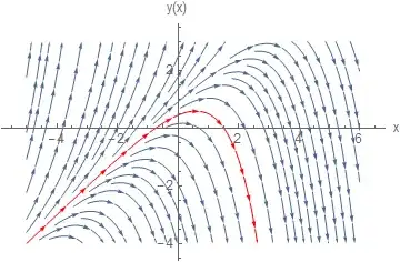
One direct way, is to use Show and simply add the solution to the Stream plot. Here is a quick example (since you did not give one)

f[x_, y_] := y - x
p1 = StreamPlot[{1, f[x, y]}, {x, -5, 6}, {y, -4, 3}, Frame -> False, 
   Axes -> True, AspectRatio -> 1/GoldenRatio, 
   AxesLabel -> {"x", "y(x)"}, BaseStyle -> 12]

Now to add solution curve, use DSolve to find the solution and add it using Show

ic = y[1] == .5;
sol = y[x] /. First@DSolve[{y'[x] == y[x] - x, ic}, y[x], x];
p2 = Plot[sol, {x, -4, 6}, PlotStyle -> Red];
Show[p1, p2]

Second method

Use the option StreamPoints to select stream line, which passes through the initial conditions. This is automatically then the solution curve. This does not require one to solve the ODE and obtain the solution like the above.

f[x_, y_] := y - x
p1 = StreamPlot[{1, f[x, y]}, {x, -5, 6}, {y, -4, 3}, Frame -> False, 
  Axes -> True, AspectRatio -> 1/GoldenRatio, 
  AxesLabel -> {"x", "y(x)"}, BaseStyle -> 12, 
  StreamPoints -> {{{{1, .5}, Red}, Automatic}}]

Answer 2

Here is another way to super impose solution curves on the stream lines. For this I choose a random IVP.

Random example

soln[y0_?NumericQ]:=First@NDSolve[{y'[x] == -1 + Sin[y[x]], y[0] == y0}, {y}, {x, -10,10}];
sp = StreamPlot[{1, (-1 + Sin[y])}, {x, -3, 3}, {y, -3, 3}];
Show[sp, Plot[Evaluate[{y[x]} /. soln[#] & /@ Range[-20, 20, 0.3]], {x, -3, 3}, 
  PlotRange -> All, MaxRecursion -> 8, AxesLabel -> {"x", "y"},PlotStyle -> Red]]

OP's system

sp = StreamPlot[{-2*x + y - 11, -5*x + 4*y - 35}, {x, -15,15}, {y, -20, 20}];

soln[x0_?NumericQ] := 
  First@NDSolve[{x'[t] == -2*x[t] + y[t] - 11, x[0] == x0, 
     y'[t] == -5*x[t] + 4*y[t] - 35, y[0] == x0}, {x, y}, {t, -20, 5}];

Show[sp, ParametricPlot[Evaluate[{x[t], y[t]} /. soln[#] & /@ Range[-15, 15, 1]], {t, -15, 
   5}, PlotRange -> All, MaxRecursion -> 8, AxesLabel -> {"x", "y"},PlotStyle -> Red]]