Compute the curvature of a bent stack of paper

Question

My goal is to link the curvature of a bent stack of paper in a wind tunnel to its bending modulus $B$, knowing all the other physical properties. To this end, I would like to reproduce the numerical simulation in P. Buchak, C. Eloy and P. M. Reis, Phys. Rev. Lett. 105, 194301 (2010), also available here.

With $s$ the curvilinear abscissa along the stack, and $\theta(s)$ the angle between the stack and horizontal at $s$, the curvature of the stack should be governed by:

Fx'[s] == 
  -rhoa*U^2*W*Sin[theta[s]]*(N[Pi,10]/4*W*Cos[theta[s]]^2*theta'[s] - 
    0.5*Cd*Sin[theta[s]]^2)

Fy'[s] == 
  -rhoa*U^2*W*Cos[theta[s]]*(0.5*Cd*Sin[theta[s]]^2 - 
    N[Pi,10]/4*W*Cos[theta[s]]^2*theta'[s])+sigmap*9.81*W

B*W*theta''[s] == Sin[theta[s]]*Fx[s] - Cos[theta[s]]*Fy[s]

with the following boundary conditions:

Fx[L] == 0,Fy[L] == 0,theta[0] == 0,theta'[L] == 0

where $L$ is the length of the stack.

The other parameters are: $U$ (wind speed), $\rho_a$ (density of air), $W$ (stack width), $C_d$ (drag coefficient), $\sigma_p$ (area density of stack) — all of which I know experimentally — and $B$ (bending modulus) which I am looking for.

I tried to compute these equations using Mathematica's NDSolve.

sol = 
  NDSolve[{(*equations*),(*boundary conditions*)}, {Fx, Fy, theta}{s, 0, L},
    MaxSteps -> Infinity, InterpolationOrder-> All];

and plotted the expected shape of the stack.

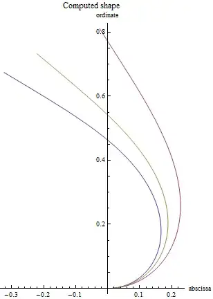
The result is that... it doesn't match at all! (the following figures correspond to $U=5m\cdot s^{-1}$)

Furthermore, the code can lead to very surprising results for high wind speed! (the following figure corresponds to $U = 10m\cdot s^{-1}$ and $L = 0.3m$, all the other parameters being unchanged)

Are there other computational methods which would work to solve this ODE system, or more efficient and accurate options to use with NDSolve?

-------- EDIT --------

As requested, I provide here a complete Mathematica code.

The governing equations of my system can be rewritten as

Fx'[s] == Sin[theta[s]](0.5*Cd*Cy*Sin[theta[s]]^2-
        0.25*N[Pi,10]*lambda*Cy*Cos[theta[s]]^2*theta'[s])
Fy'[s] == -Cos[theta[s]](0.5*Cd*Cy*Sin[theta[s]]^2-
       0.25*N[Pi,10]*lambda*Cy*Cos[theta[s]]^2*theta'[s])+Delta
theta''[s] == Sin[theta[s]]*Fx[s]-Cos[theta[s]]*Fy[s]

and have the same boundary conditions as previously.

The algorithm now has 4 adimensionned parameters: $C_d = 1.76$ (drag coefficient), $C_y = \frac{\rho_aU^2L^3}{B}$ (Cauchy number, $C_y > 18.5$), $\lambda = \frac{W}{L}$ (aspect ratio, $0.1 < \lambda < 0.5$) and $\Delta = \frac{\sigma_pgL^3}{B}$ (elastrogravity number, $0.1 < \Delta < 20$).

(* PARAMETERS *)
Cd = 1.76; (* drag coefficient *)
Cy = 90; (* Cauchy number *)
lambda = 0.4; (* aspect ratio *)
Delta = 1; (* elastogravity number *)

(* SIMULATION *)
sol = NDSolve[{Fx'[s]==Sin[theta[s]](0.5*Cd*Cy*Sin[theta[s]]^2-
               0.25*N[Pi,10]*lambda*Cy*Cos[theta[s]]^2*theta'[s]),
               Fy'[s]==-Cos[theta[s]](0.5*Cd*Cy*Sin[theta[s]]^2-
               0.25*N[Pi,10]*lambda*Cy*Cos[theta[s]]^2*theta'[s])+Delta,
               theta''[s]==Sin[theta[s]]*Fx[s]-Cos[theta[s]]*Fy[s],
               Fx[1]==0,Fy[1]==0,theta[0]==0,theta'[1]==0},{Fx,Fy,theta},
               {s,0,1},MaxSteps->Infinity,InterpolationOrder->All];
(* résolution du système *)

(* PLOT *)
ParametricPlot[{Integrate[Cos[Evaluate[theta[t] /. sol][[1]]], {t,0,s}],
                Integrate[Sin[Evaluate[theta[t] /. sol][[1]]],{t,0,s}]},
               {s, 0, 1},AspectRatio->1,AxesLabel->{"abscissa","ordinate"},
               PlotLabel->"Computed shape"]

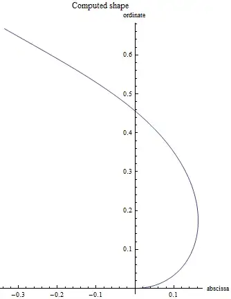
The (* PLOT *) section returns a graph of the computed shape of the stack (ie, $y = \int_0^1 ds \sin(\theta)$ vs. $x = \int_0^1 ds \cos(\theta)$).

Executing this script gave me the following graph

which does not match the experimental observations (see 1st figure of the question).

Thanks for your help!

Answer 1

yketa's guess is right. This nonlinear boundary value problem (BVP) has multiple solutions, and we need to manually set proper initial guess for "Shooting" method to get the desired result. Let me reproduce FIG.2 in the paper:

(* Parameters are taken from the paper. *)
Ulst = {111/10, 65/10, 88/10};
g = 981/100;
rhoa = 129/100;
L = 15 10^-2;
W = 29/10 10^-2;
BW = 24 10^-5;
rhophW = 114/1000/10^3 10^2;
rhoph = rhophW/W;
B = BW/W;
Delta = rhoph g L^3/B;
lambda = W/L;
Cd = 176/100;
Cy = rhoa U^2 L^3/B;

k = 1/2 Cd Cy Sin[theta[s]]^2 - Pi/4 lambda Cy Cos[theta[s]]^2 theta'[s];

(* The integration can be computed inside NDSolve, too. *)
add = {intSin'[s] == Sin@theta[s], intSin[0] == 0, intCos'[s] == Cos@theta[s], 
   intCos[0] == 0};

Clear[sol, U]
shoot[ic_] := {"Shooting", "StartingInitialConditions" -> ic};
sol[var_] := Block[{U = var}, First@NDSolve[{
      Fx'[s] == Sin[theta[s]] k,
      Fy'[s] == -Cos[theta[s]] k + Delta,
      theta''[s] == Sin[theta[s]] Fx[s] - Cos[theta[s]] Fy[s],
      Fx[1] == 0, Fy[1] == 0, theta[0] == 0, theta'[1] == 0, add}, 
       {Fx, Fy, theta, intSin, intCos}, {s, 0, 1}, 
     Method -> shoot@{Fx[1] == 0, Fy[1] == 0, theta[1] == 3, 
        theta'[1] == 0, intSin[1] == 0, intCos[1] == 0}]];

ParametricPlot[{intCos@s, intSin@s} /. sol /@ Ulst // Evaluate, {s, 0, 1}, 
 AxesLabel -> {"abscissa", "ordinate"}, PlotLabel -> "Computed shape"]

---

In the code piece above, I simply dope out the proper initial guess intuitively, but this can actually be done in a systematic way for your problem. Let me show you the way with the parameters given in your question as an example.

We first set up a initial value problem with ParametricNDSolveValue:

Cd = 1.76;(*drag coefficient*)
Cy = 90;(*Cauchy number*)
lambda = 0.4;(*aspect ratio*)
Delta = 1;(*elastogravity number*)
k = 1/2 Cd Cy Sin[theta[s]]^2 - Pi/4 lambda Cy Cos[theta[s]]^2 theta'[s];
add = {intSin'[s] == Sin@theta[s], intSin[0] == 0, intCos'[s] == Cos@theta[s], 
   intCos[0] == 0};
test = ParametricNDSolveValue[{
    Fx'[s] == Sin[theta[s]] k,
    Fy'[s] == -Cos[theta[s]] k + Delta,
    theta''[s] == Sin[theta[s]] Fx[s] - Cos[theta[s]] Fy[s],
    Fx[1] == 0, Fy[1] == 0,(*,theta[0]\[Equal]0*)theta[1] == par, 
    theta'[1] == 0}, {Fx, Fy, theta}, {s, 0, 1}, par];

Then we need to find out all the possible values of par that result in theta[0] == 0. (It is not hard for your specific problem because 0 < par <2 Pi according to the model. ) This job can be done by e.g. RootSearch, but here I'll just do it in a more basic way i.e. by observing the graph:

Plot[test[par][[3]][0], {par, 0, 2 Pi}, PlotRange -> 1]

From the graph we can see 3 (4?) possible solutions. We try them from right to left:

rst = NDSolve[{
    Fx'[s] == Sin[theta[s]] k,
    Fy'[s] == -Cos[theta[s]] k + Delta,
    theta''[s] == Sin[theta[s]] Fx[s] - Cos[theta[s]] Fy[s],
    Fx[1] == 0, Fy[1] == 0, theta[0] == 0, theta'[1] == 0, add}, {Fx, Fy, 
    theta, intSin, intCos}, {s, 0, 1}, 
   Method -> shoot@{Fx[1] == 0, Fy[1] == 0, theta[1] == 2.6, 
      theta'[1] == 0, intSin[1] == 1, intCos[1] == 1}];

ParametricPlot[{intCos@s, intSin@s} /. rst // Evaluate, {s, 0, 1}, 
 AxesLabel -> {"abscissa", "ordinate"}, PlotLabel -> "Computed shape"]

OK, the right-most root is the one we need.