One way to solve this is to ask Mathematica to solve it for general boundary conditions, and then specialize to the case you're actually interested in:
ClearAll[Y, Bb, t]
Y[t_] = Y[t] /. DSolve[{Y'[t] == Sqrt[Y[t]] - Bb, Y[0] == Cc^2}, Y, t] // Simplify;
Y[t] /. Cc -> Bb
N[% /. t -> 0]

(* {Bb^2 (1 + ProductLog[-2 E^((-4 Bb + t)/(2 Bb))])^2, Bb^2} *
(* {0.35239 Bb^2, Bb^2} *)
The first solution here is the one you already found. The second one is new, and is in fact a valid solution for the initial conditions $y(0) = B$.
In fact, the only valid solution of your equation with the initial conditions $y(0) = B$ is $y(t) = B$. This can be seen by performing a separation of variables and integrating; we obtain the implicit solution
$$
2 (\sqrt{y} - \sqrt{y_0}) - 2 B \ln \left(\frac{\sqrt{y} - B}{\sqrt{y_0} - B} \right) = t,
$$
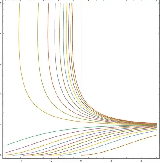
where we use the general boundary condition $y(0) = y_0$. It can easily be seen that this equation cannot be satisfied if $y_0 = B^2$. (The separation-of-variables method assumes that $\sqrt{y} - B \neq 0$, so the trivial solution evades this problem.) Plotting the above contours for $B = 1$ also makes it pretty evident that the only solution for $y(0) = B$ is the trivial solution $y(t) = B$.
ContourPlot[Evaluate[Table[2 (Sqrt[y] - Sqrt[y0]) - 2 Log[(Sqrt[y] - 1)/(Sqrt[y0] - 1)] == x, {y0, -2, 2, 0.1}]], {x, -5, 5}, {y, 0, 5},
  PlotPoints -> 100, ImageSize -> Large, Axes -> True]