24

I would like to show the iterative stages of infection for problem 2 in this link.

In case the link dies, I have copied the text for the problem below:

One hundred computers are connected in a 10x10 network grid, as below. At the start exactly nine of them are infected with a virus. The virus spreads like this: if any computer is directly connected to at least 2 infected neighbours, it will also become infected.

It is fairly straightforward to show the first stage of infection (blue):

Module[{a, b, c, d, e, x, y, z},

x = 6; y = 5;
z = Array[{#, #2} &, {y, y}];
a = Flatten[z, 1];
b = RandomSample[a, x];
c = Complement[a, b];
d = Select[
    Thread@{c, Thread@Table[EuclideanDistance[b[[t]], #] & /@ c, {t, x}]}, 
    Count[#[[2]], 1] > 1 &][[All, 1]];
e = Complement[a, Join[b, d]];

Graphics[{Line /@ Join[z, Thread@z], PointSize[.05], 
Point /@ e, Red, Point /@ b, Blue, Point /@ d}]

]

I would like to show (via manipulate or otherwise) each stage of infection until the maximum number for that particular seed has been infected. I have had a play with NestWhileList, but coming up short at present.

Mr.Wizard
  • 271,378
  • 34
  • 587
  • 1,371
martin
  • 8,678
  • 4
  • 23
  • 70

3 Answers3

37

If it is at all an option to represent the grid as a 2D list instead of a list of infected coordinates, I would model this is a cellular automaton. What you've essentially got is an outer totalistic cellular automaton with a von Neumann neighbourhood. The rule in Game-of-Life notation is B234/S01234, i.e. a cell comes to life if it has two or more live neighbours and it always survives. Implementing simple CAs is quite straight-forward with Mathematica's CellularAutomaton, and I've written another answer here about how to figure out the rule number of the CA.

For your case, we're using the weights:

{{0, 2, 0}, 
 {2, 1, 2}, 
 {0, 2, 0}}

And then the rule turns out to be 1018. So we can simulate a single step with the following function:

CellularAutomaton[
  {
    1018, 
    {2, {{0, 2, 0}, {2, 1, 2}, {0, 2, 0}}}, {1, 1}
  }, 
  {#, 0}
][[1, 2 ;; -2, 2 ;; -2]] &

The indexing at the end is used to remove the background information returned by CellularAutomaton.

However, as of version 11.1 specifying common CA rules has become a lot more convenient. The possibility to specify a CA rule via an association allows for rather high-level classifications. In fact, Mathematica now knows about various neighbourhoods:

CellularAutomaton[<|
    "OuterTotalisticCode" -> 1018, 
    "Neighborhood" -> "VonNeumann", 
  |>, 
  {#, 0}
][[1, 2 ;; -2, 2 ;; -2]] &

And we don't even need to compute that rule code, because we can specify the rule directly via a set of growth cases:

CellularAutomaton[<|
    "GrowthCases" -> {2, 3, 4}, 
    "Neighborhood" -> "VonNeumann", 
  |>, 
  {#, 0}
][[1, 2 ;; -2, 2 ;; -2]] &

This says "when a dead cell has 2, 3 or 4 live neighbours, the cell comes alive", which is exactly what we're looking for.

To simulate the infection to convergence, I'd recommend FixedPointList instead of NestWhileList. It simply applies a function over and over until the value stops changing, and then gives you all the intermediate values.

Module[{a, b, d = 25},
  a = RandomChoice[{0, 0, 0, 0, 0, 0, 0, 1}, {d, d}];
  b = Most @ FixedPointList[
    CellularAutomaton[<|
        "GrowthCases" -> {2, 3, 4}, 
        "Neighborhood" -> "VonNeumann", 
      |>, 
      {#, 0}
    ][[1, 2 ;; -2, 2 ;; -2]] &, a];
  ListAnimate[ArrayPlot /@ b]
]
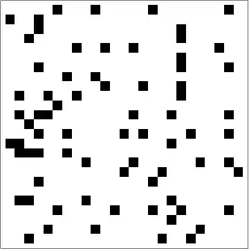
enter image description here

Adding some information about the history is as easy as calling Accumulate on the list of grids before handing them to ArrayPlot, which now colours each cell by its relative age:

enter image description here

To show the absolute age instead of the relative age, you can give ArrayPlot the option PlotRange -> {0, Length@b}:

enter image description here

Martin Ender
  • 8,774
  • 1
  • 34
  • 60
12

Non CellularAutomaton solution, using @MartinEnder's suggestion of FixedPointList as opposed to NestWhileList:

f[initial_List, infected_List, rest_List] := 
  With[{newinfected = Join[infected, Select[Thread@{rest, 
  Thread@Table[EuclideanDistance[infected[[t]], #] & /@ rest, 
  {t, Length@infected}]}, Count[#[[2]], 1] > 1 &][[All, 1]]]}, 
  {initial, newinfected, Complement[initial, newinfected]}];

z = Array[{#, #2} &, {10, 10}]; a = Flatten[z, 1];
b = {{1, 1}, {1, 10}, {3, 3}, {4, 5}, {4, 7}, {5, 8}, {7, 5}, {7, 10}, {9, 9}, {10, 4}};
c = Complement[a, b];

With[{e = FixedPointList[f[#[[1]], #[[2]], #[[3]]] &, {a, b, c}]}, 
Manipulate[Graphics[{Thickness[.01], Line /@ Join[z, Thread@z], PointSize[.05], 
RGBColor[0, .5, 1], Point /@ e[[w, 3]], RGBColor[1, .5, 0], 
Point /@ e[[w, 2]]}], {w, 1, Length@e, 1}]]

martin
  • 8,678
  • 4
  • 23
  • 70
  • @AnjanKumar no, it won't for 9 on a 1010 grid. There are solutions for 10 on a 1010 grid though - like the one above. – martin Mar 16 '17 at 04:14
7

The demonstration of CellularAutomaton is impressive but it is far from necessary for this problem. I propose ListCorrelate instead. Keeping much of Martin Ender's code for ease of comparison:

d = 25;

a = RandomChoice[{7, 1} -> {0, 1}, {d, d}];

ker = {{0, 1, 0},
       {1, 2, 1},
       {0, 1, 0}};

fn = UnitStep[ListCorrelate[ker, #, 2, 0] - 2] &;

ArrayPlot /@ FixedPointList[fn, a] // ListAnimate

enter image description here

In addition to being simpler (in my opinion) ListCorrelate is somewhat faster:

ender = CellularAutomaton[{1018, {2, {{0, 2, 0}, {2, 1, 2}, {0, 2, 0}}}, {1, 
       1}}, {#, 0}][[1, 2 ;; -2, 2 ;; -2]] &;

big = RandomChoice[{20, 1} -> {0, 1}, {1000, 1000}];

Nest[ender, big, 10] // RepeatedTiming // First
Nest[fn, big, 10]    // RepeatedTiming // First
0.606

0.363

(In Mathematica 10.1 I cannot test the newer syntax shown.)

Mr.Wizard
  • 271,378
  • 34
  • 587
  • 1,371