Reduce distances between vertices of graph to minimum possible?

Question

This simple graph has vertex shapes of different sizes:

edges = {1 \[DirectedEdge] 2, 2 \[DirectedEdge] 3, 3 \[DirectedEdge] 1};
vsf[{xc_, yc_}, name_, {w_, h_}] :=
  Module[{},
   Switch[name,
    1, size = 0.1,
    2, size = 0.2,
    3, size = 0.3];
   Disk[{xc, yc}, size]
   ];
Graph[edges, VertexShapeFunction -> vsf, VertexLabels -> edges]

So now I want to reduce the distance between the vertices according to the size of the shapes:

It's like the edges are elastic. Perhaps there's some kind of layout option that does this that I can't find, or some way of allowing the edges to be controlled by the vertex shape function? I'm struggling with Mathematica 8 graphing a bit, to be honest (is it just me, or is the documentation not up to the usual standards?) so I don't know whether this is possible, difficult, or easy...

I'm hoping to be able to use graph/network tools to produce images like this (see the interactive version here:

and also apply a similar technique to other ideas, such as this graph for the US 2012 election:

Answer 1

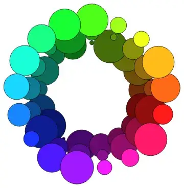
This is a form of anamorphic map or cartogram. (For an early account of how people made such things manually, see http://qmrg.org.uk/files/2008/11/59-area-cartograms.pdf; page 35 shows two examples with circular figures.)

Such maps are made by optimizing an objective function. The function must express

• The amount of distortion in shape and position of the features and

• The degree to which the areas of the features are proportional to the desired size.

In this instance there is no question of optimizing the distortion of shape, because all shapes on the map will be the same: that is not going to vary. We may dispense with the second part of the objective (if we like) by insisting that the circle areas be directly proportional to the desired sizes, without error. That leaves only the first objective: minimizing the dislocation of the feature positions.

Here is the kind of thing we're aiming for: converting this

(plus size information for the vertices) into this:

(In this example, features that were edge-adjacent in the abstract graph are spatially adjacent, or nearly so insofar as that is possible, and most features do not overlap--but some evidently do.)

As a constraint, we would like the features not to overlap. To achieve some flexibility, I propose dealing with this via a penalty function: add a term to the objective function that increases with the amount of overlap. By choosing a suitable form of the objective, that will make this an unconstrained differentiable program, which is relatively straightforward to solve numerically. It will, unfortunately, have many local minima.

I have included some parameters to control how the penalty is balanced against the original objective.

For the original objective we can look at all pairs of features that are supposed to be adjacent, compare their actual distances to the desired distances, and attempt to minimize some function of this that will be zero when the two values agree. The square of the discrepancy is simple to compute and well-behaved (differentiable, etc.).

For the penalty we can do the same thing but (a) we need to look at all pairs of features and (b) there should be no penalty when there is no overlap. To provide flexibility, my code uses a user-settable power of the discrepancy in distances when there is overlap and multiplies that by a user-settable constant. Both these parameters control how the objective balances getting adjacent features close against preventing overlap of all features. A little experimentation typically produces acceptable solutions. Increasing the multiple prevents overlap well. Increasing the power prevents severe overlap but permits small amounts of overlap.

In the following I have made no effort to speed the solutions, but the usual ways should work, especially compiling the objective function. $100$ iterations (on one core) of my machine take $30$ seconds and usually Mathematica halts then with a message saying the solution hasn't converged. It doesn't seem to matter: it gets pretty good results anyway.

(One way to do better is with a simulated annealing solution.)

The code is contained in the function anamorph. Its arguments are a list of desired vertex sizes (as final radii of the circles), an adjacency matrix (which could be weighted if desired), an "exclusion" matrix which typically should have unit values off the diagonal and zeros on the diagonal (and also can be weighted), a set of starting vertex coordinates, and the penalty parameters strength and power. Providing a set of starting coordinates is important in order to "steer" the solution towards a local minimum that approximates a good initial configuration. (It is too much to hope that numerical methods will always find a global minimum for this problem, at least when the graph has many vertices and edges.)

anamorph[sizes_, adjacency_, exclusion_, start_, {strength_: 1, power_: 2}] := 
  Module[{vars, objective1, objective2, soln, shape, x},
   vars = Table[{Unique[x], Unique[y]}, {Length[sizes]}];
   objective1[x_] := 
    With[{y = 
       Flatten[adjacency (Outer[(#1 - #2).(#1 - #2) &, x, x, 1] - 
           Outer[Plus, sizes, sizes]^2)]}, y.y] ;
   objective2[x_] := 
    With[{y = 
       Flatten[exclusion (Outer[(#1 - #2).(#1 - #2) &, x, x, 1] - 
           Outer[Plus, sizes, sizes]^2)]},
      Sum[Boole[z < 0] (-z)^power, {z, y}]] ;
   soln = 
    FindMinimum[objective1[vars] + strength objective2[vars], 
     Evaluate @ Transpose[Flatten /@ {vars, start}]];
   shape[x_List, v_, ___] :=  Disk[x, sizes[[ToExpression[v]]]];
   x =  vars /. Last[soln];
   {objective1[x], objective2[x], 
    AdjacencyGraph[adjacency, VertexCoordinates -> x, 
     VertexShapeFunction -> shape, EdgeStyle -> Opacity[0]]}
   ];

It returns a list of three things: the value of the original objective function, the value of the penalty function, and a Graph object showing the solution. The first two numbers are valuable for comparing solutions; ideally they should both be zero, but in fact they usually cannot both simultaneously be zero. That's where the tradeoffs come in.

As an example of its use, consider this graph endowed with random vertex sizes. (I obtain starting coordinates by first creating the abstract adjacency graph and extracting the vertex coordinates from that.)

styles  = Flatten[Table[17 i + j -> Hue[j/17, .9, (i^2 + 3)/7], {i, 0, 2}, {j, 1, 17}]] ;
g = GraphData[{"Web", 17}]; n = VertexCount[g];
a = AdjacencyMatrix[g];
e = ConstantArray[1, {n, n}] - IdentityMatrix[n];
s = RandomReal[{0.001, 1}, n] // Sqrt;
start =  (AbsoluteOptions[g, VertexCoordinates] // Last) // Chop;
g = AdjacencyGraph[a, VertexStyle -> styles];

It is drawn below. But first, here is an anamorphic solution intended to have little or no overlap, as prescribed by setting strength to $100$:

{time, {o1, o2, gg}} = AbsoluteTiming[anamorph[s, a, e, start, {100, 2}]]

It takes 30 seconds. The values of the two parts of the objective function are $458$ and $0.25$ for the original objective and the penalty, respectively, showing that some vertices will not be perfectly adjacent but that there is little overlap.

(The default application of anamorph with strength set to $1$ produced the graph shown near the beginning of this answer. The value of the objective function is just $20$, much lower than $458$, expressing a fairly close correspondence between spatial proximity in the image and adjacency in the original graph, but it has perhaps too much overlap, as expressed by a value of $27.7$ instead of $0.25$ for the penalty. You pick your poison...)

Let's look at the original and transformed graphs:

AdjacencyGraph[a, 
 Options[gg, {VertexShapeFunction}], VertexStyle -> styles, EdgeStyle -> Opacity[0]]

AdjacencyGraph[a, 
 Options[gg, {VertexShapeFunction, VertexCoordinates}], 
 VertexStyle -> styles, EdgeStyle -> Opacity[0]]

Evidently the result is rotated relative to the original. We could prevent this by pinning down one of the vertex coordinates (not letting it vary from its start) and constraining its direction towards another vertex. Another way is to add a term to the objective function equal to the sum of squared displacements of the vertices from their start positions. (I don't like this because the start positions might have too much influence in the final answer, but it has its place as a Dorling cartogram; the link shows a dynamic animation of a solution.) It perhaps is easiest just to rotate the result as you see fit so it more closely matches the original image.