System of ODEs specified by large coefficient matrices

Question

What is the best way to call NDSolve for solving a system of differential equations of the form

Am.y'[x] + Bm.y[x]/x + Cm.y[x] == Dv

with y[0] == Ev in the interval x from 0 to 1.

where y is an n-vector, Am, Bm, and Cm are n x n coefficient matrices, and Dv and Ev are n vectors. Say with

n=100;
Am = RandomReal[1,{n,n}];
Bm = RandomReal[1,{n,n}];
Cm = RandomReal[1,{n,n}];
Dv = RandomReal[1,{n}];
Ev = RandomReal[1,{n}];

Related: http://mathematica.stackexchange.com/q/14407/57 – Sjoerd C. de Vries Nov 25 '12 at 20:18 — Sjoerd C. de Vries, Nov 25 '12 at 20:18
You also need sufficient initial and boundary conditions – Sjoerd C. de Vries Nov 25 '12 at 20:41 — Sjoerd C. de Vries, Nov 25 '12 at 20:41

score 2 · Accepted Answer · answered Nov 26 '12 at 01:03

Here is an example with some small matrices, but it's the same for large ones. The key point is to use the NDSolve option SolveDelayed->True

Some system matrices:

matS = {{0, 0, 0, 0, 0, 0}, {0, 0, 0, 0, 0, 0}, {0, 0, 0, 0, 0,
         0}, {0, 0, 0, 0, 0, 0}, {0, 0, 0, 0, 0, 0}, {0, 0, 0, 0, 0, 
    0}};

matD = {{0, 0, 0, 0, 1, 0}, {0, 1/1000, 0, -(1/1000), 0, 0}, {0, 0, 
    1,0, 0, 0}, {0, -(1/1000), 0, 1/1000, 0, -1}, {1, 0, 0, 0, 0,
         0}, {0, 0, 0, -1, 0, 0}};

matM = {{1/1000000, -(1/1000000), 0, 0, 0, 0}, {-(1/1000000), 1/
          1000000, 0, 0, 0, 0}, {0, 0, 0, 0, 0, 0}, {0, 0, 0, 0, 0, 
    0}, {0,
         0, 0, 0, 0, 0}, {0, 0, 0, 0, 0, 0}};

matL = {0, 0, 0, 0, 5 (1/2 + 1/2 Erf[100000 (-(1/1000) + t)]), 0};

sysSize = Length[matS];
tInit = 0.;
tEnd = 0.01;
init = Table[0, {sysSize}];
dinit = LinearSolve[matD, -(matS.init - matL) /. t -> tInit];

if = u /.First /@ NDSolve[{matM.Derivative[2][u][t]+matD.Derivative[1][u][t] + matS.u[t] == matL, u[tInit] == init,Derivative[1][u][tInit]==dinit}, u, {t, tInit, tEnd},SolveDelayed->True]

The interpolation function then returns a vector for a time t:

if[0.001]
(*
{0.00001410474097541479`, 0.000014042475237194534`, 0.`, 0.`, -1.4042475237194535`*^-8, -1.4042475237194532`*^-8}
*)

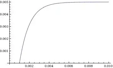
To plot it:

Plot[if[t][[2]], {t, tInit, tEnd}]

enter image description here

If your coefficient matrices are functions, then you can use matD[x] and make a function like matD[x_?VectorQ]:=... or some other appropriate pattern.

Here is an example for larger system matrices.

score 0 · Answer 2 · answered Nov 25 '12 at 22:31

This system of differential equations has the form: $$ x \frac{\mathrm{d}}{\mathrm{d}x} \left( \hat{A} \cdot \vec{y}(x) \right) + \left( x \hat{C} + \hat{B} \right) \cdot \vec{y}(x) = x \vec{D} \tag{1} $$ Notice that $x=0$ is the singular point of the system, hence the initial value problem eq.(1) and $\vec{y}(0) = \vec{E}$ is not well defined, because the fundamental system of eq. (1) becomes degenerate at $x=0$.

Frobenius method can be used to construct a series approximation: $$ \vec{y}(x) = \vec{E} + \vec{F}_1 x + \vec{F}_2 \frac{x^2}{2} + \mathcal{o}\left(x^2\right) $$ Substituting back into eq. (1) we discover: $$ \hat{A} \cdot \vec{F}_1 x + 2 \hat{A} \cdot \vec{F}_2 \frac{x^2}{2} + \mathcal{o}\left(x^2\right) + \left(\hat{B} \cdot \vec{E}+ x \left( \hat{C} \cdot \vec{E} + \hat{B} \cdot \vec{F}_1 \right) + \frac{x^2}{2} \left(2 \hat{C} \cdot \vec{F}_1 + \hat{B} \cdot \vec{F}_2 \right) + \mathcal{o}\left(x^2\right) \right) = x \vec{D} $$ Comparing terms we get: $$\begin{eqnarray} \hat{B} \cdot \vec{E} &=& \vec{0} \\ \left(\hat{A} + \hat{B}\right) \cdot \vec{F}_1 + \hat{C} \cdot \vec{E} &=& \vec{D} \\ \left(2 \hat{A} + \hat{B}\right) \cdot \vec{F}_2 + 2 \hat{C} \cdot \vec{F}_1 &=& \vec{0} \end{eqnarray} $$ Assuming consistency and solvability of the above, we can approximate $y(x)$ away from the origin $x=0$, and then call NDSolve to solve a well-defined initial value problem.

System of ODEs specified by large coefficient matrices

2 Answers2

Linked