Fitting a polynomial: choose a good basis
Let's look at the function:
Plot[Cs[x]/Cp[x], {x, 0, 1}, PlotRange -> All]

It doesn't look much like a polynomial, except perhaps like the flipped-around graph of x^1000.
Let's try something like that:
With[{r = 1.02},
 lmf = LinearModelFit[
   SetPrecision[Table[{r^p, Cs[r^p]/Cp[r^p]}, {p, -800, 0}],
    MachinePrecision],
   Table[(1 - x)^(200 n), {n, 26}],
   x
   ]
 ]
Error is not bad, but one could hope for better:
Plot[Cs[x]/Cp[x] - lmf[x] // Evaluate, {x, 0, 1}, PlotRange -> All]

The coefficients are given by
lmf@"BestFitParameters"
The coefficients are quite frightening numerically, many between 10^6 and upwards of 10^8 and alternating signs. Note that the basis functions (1 - x)^k should never be expanded, since k ranges up to over 5000.
Chebyshev approximation
According to Weierstrass, there should be no limit to how well we can approximate (at least with exact coefficients and inputs). Chebyshev interpolations typically are robust, but we will see that does not make it easy to approximate the OP's funcion. The function chebSeries below computes the degree n series of Chebyshev coefficients of the Chebyshev polynomials of the interpolation through the Chebyshev points (x in the code):
chebSeries[f_, a_, b_, n_, prec_ : MachinePrecision] :=
 Module[{x, y, cc},
  x = Rescale[Sin[N[(π Range[n, -n, -2])/(2 n), MachinePrecision]], {-1, 1}, {a, b}];
  y = f /@ x;
  cc = Sqrt[2/n] FourierDCT[y, 1];
  cc[[{1, -1}]] /= 2; cc]
Let's do an interpolation of degree 2048, which is not a whole lot more than is needed in this case:
cc = chebSeries[x \[Function] Cs[x]/Cp[x], 0, 1, 2^11];
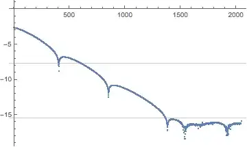
As the order of the interpolation increases, the coefficients of the interpolation approach the (infinite) Chebyshev series expansion of the function. The error of a truncated series is at most the sum of the absolute values of the lopped-off coefficients. For a nice function, these coefficients eventually converge exponentially to zero, which is the case here:
ListPlot[RealExponent@cc,
 GridLines -> {None, Log10[Max[Abs@cc] $MachineEpsilon] {1/2, 1}}]
We can get an numerical estimate of the error of truncation from the coefficients themselves:
cc[[510 ;; 513]]
cc[[-4 ;;]]
(*
  {-9.30101*10^-8, 9.18019*10^-8, -9.05997*10^-8, 8.94039*10^-8}
  {-5.89806*10^-17, 5.26922*10^-17, -5.37764*10^-17, 1.11022*10^-16}
*)
The corresponding polynomial (truncated series of degree n) is given by
With[{coeffs = cc[[ ;; n+1]]},
 coeffs.ChebyshevT[Range[0, Length@ coeffs - 1], 1 - 2 x]
]
We can get almost machine precision this way. Let's begin by estimating the error by summing the tail, for both single and double precision accuracy, and calculate the number of terms of the Chebyshev series needed to obtain the desired precisions.
single = Length@cc -
  Module[{sum = 0.}, LengthWhile[Reverse@cc, (sum += #) < Sqrt@$MachineEpsilon/2 &]]
double = Length@cc -
  Module[{sum = 0.}, LengthWhile[Reverse@cc, (sum += #) < $MachineEpsilon &]]
(*
  617
  1535
*)
The function cheval evaluates a given Chebyshev series with coefficients cc over the interval {a, b}. The argument to ChebyshevT needs to be rescaled to run from -1 to 1 as x runs from a to b. It is also important that ChebyshevT[] not evaluate on symbolic x, because it will evaluate to a polynomial in powers of x, which will be numerically unstable to evaluate, especially at such extremely high degrees as we have.
Simplify@Rescale[x, {a, b}, {-1, 1}]
(*  (a + b - 2 x)/(a - b)  *)

ClearAll[cheval];
cheval[x_?NumericQ, a_?NumericQ, b_?NumericQ, cc_] :=
  cc.ChebyshevT[Range[0, Length@cc - 1], (a + b - 2 x)/(a - b)];
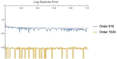
Here is a plot of the logarithm of the absolute error of the "single" and "double" precision series. We see that it is possible to achieve single precision accuracy (when computing with double precision floats), but the double precision series sometimes has small but noticeable rounding errors.
Plot[Cs[x]/Cp[x] - {cheval[x, 0, 1, cc[[;; single]]],
     cheval[x, 0, 1, cc[[;; double]]]} // RealExponent // Evaluate,
 {x, 0, 1},
 PlotLabel -> "Log Absolute Error", MaxRecursion -> 2,
 PlotLegends -> {Row[{"Order ", single - 1}], Row[{"Order ", double - 1}]},
 PlotRange -> {0, -19},
 GridLines -> {None, Log10[Max[Abs@cc] $MachineEpsilon] {1/2, 1}}]
The OP stated than a polynomial approximation was desired. Chebyshev series are probably the best way to do it easily, but their degrees might be prohibitive.
Piecewise Chebyshev approximation
Finally, piecewise interpolation will make it easier to have small degrees, and in Mathematica the inconvenience of piecewise functions is small.
The following divides the interval {0, 1} at 2^n for n = -1, -2,..., -14 and forms the degree-16 Chebyshev interpolation over each subinterval.
pwf = Piecewise@
   Join[{{cheval[x, 0, 2^(-14),
       chebSeries[x \[Function] Cs[x]/Cp[x], {0, 2^(-14)}, 16]],
      0 <= x <= 2^(-14)}},
    Table[{cheval[x, 2^(n - 1), 2^(n),
       chebSeries[x \[Function] Cs[x]/Cp[x], {2^(n - 1), 2^(n)}, 16]],
       2^(n - 1) <= x <= 2^(n)}, {n, -13, 0}]
    ];
Here is a plot of the logarithm of the absolute error. We quite easily get near machine precision accuracy.
Plot[Cs[x]/Cp[x] - pwf // RealExponent // Evaluate,
 {x, 0, 1},
 PlotLabel -> "Log Absolute Error", PlotRange -> {-13, -17},
 GridLines -> {None, Log10[Max[Abs@cc] $MachineEpsilon] {1/2, 1}}]

One could also use chebInterpolation to construct an InterpolatingFunction instead of a Piecewise function. Both can be used inside NDSolve.


