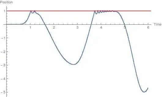
I am simulating the dynamics of a spring mass system impact an obstacle. I will not go into the details of the numerical scheme, but here are the general parameters and functions:
n = 10;
m = 1/n*IdentityMatrix[n];
k = n*SparseArray[{{i_, j_} /; Abs[i - j] == 1 -> -1, {i_, i_} /;
        i != n -> 2, {n, n} -> 1}, {n, n}] // Normal;
c = 0.02*k;
F0 = 10;
e = 1;
d = 1;
T = 3.4;
h = 0.002;
theta = .5;
mhat = m + h*theta*c + h^2*theta^2*k;
mhatinv = Inverse[mhat];
Fext[i_] := {F0*Cos[2 Pi/T*h*i]}~Join~ConstantArray[0, n - 1];
prox[x_, b_] := Piecewise[{{-b, x < d}, {Min[0, -b], x >= d}}]
Then I define the following 3 sequences:
Clear[ulist, vlist, vfree];

ulist[0] = ConstantArray[0, n];
vlist[0] = ConstantArray[0, n];
vfree[0] = vlist[0];

vfree[i_] := vlist[i - 1] + mhatinv.(-h*c.vlist[i - 1] - h*k.ulist[i - 1] -
     h^2*theta*k.vlist[i - 1] + h*(theta*Fext[i] + (1 - theta)*Fext[i - 1]))
ulist[i_] := ulist[i - 1] + h*(theta*vlist[i] + (1 - theta)*vlist[i - 1])
vlist[i_] := vfree[i][[;; -2]]~Join~{-e*vlist[i - 1][[-1]] + (1 + e)*
     prox[ulist[i - 1][[n]], -vfree[i][[n]]]}
Then it is possible to simulate the time-evolution of the mechanical system, and plot e.g. the trajectory of the contacting mass:
Table[ulist[i] = ulist[i]; vfree[i] = vfree[i]; vlist[i] = vlist[i], {i, 3000}];
Show[
   ListPlot[Table[{i*h, ulist[i][[n]]}, {i, 3000}]],
   Plot[1, {x, 0, 10}, PlotStyle -> Red],
   AxesLabel -> {"Time", "Position"}]
It works pretty well, however I am pretty sure this code can be improved a lot in terms of computational efficiency. I am thinking of using Compile, but it is not clear to me what to include (e.g., should the functions prox and Fext be defined in Compile? Should Compile be called for each iteration, or should the iteration process be included in it?).
Any hints would be appreciated.

memhere? Is it just a shorthand for repeating the function name inf[x_] := f[x] = rhs? – aardvark2012 Aug 15 '17 at 02:28f[x]=f[x]afterwards. Could you please elaborate a bit on that? Also, do you think it could be still possible to increase the speed significantly? – anderstood Aug 15 '17 at 15:07ulistandvlistare already packed arrays which is one sign of optimized code. – Mr.Wizard Aug 15 '17 at 17:47