NDSolve with boundary condition at infinty

Question

I have a nonlinear set of equations with a boundary condition at infinity. Consequently I have to shoot for the boundary. This question has some good ideas but there is an extra complication in my case; my boundary conditon at infinity is the second derivative going to zero and this is approached asymptotically. I will have more problems the same and this is minimum example I can demonstrate.

The equations and initial conditions at zero are here

eqns = {-Derivative[3][a[0]][η] == (-(1/2))*α*
           (-1 + 2*Derivative[1][a[0]][η]^2 + Derivative[1][a[1]][η]^2 + 
              Derivative[1][a[2]][η]^2 + Derivative[1][b[1]][η]^2 + 
              Derivative[1][b[2]][η]^2 - 
       2*a[0][η]*Derivative[2][a[0]][η] - 
              a[1][η]*Derivative[2][a[1]][η] - a[2][η]*Derivative[2][a[2]][
                  η] - b[1][η]*Derivative[2][b[1]][η] - 
              b[2][η]*Derivative[2][b[2]][η]), 
       Derivative[1][b[1]][η] - Derivative[3][a[1]][η] == 
         (1/2)*(-4*α*Derivative[1][a[0]][η]*Derivative[1][a[1]][η] - 
              2*α*Derivative[1][a[1]][η]*Derivative[1][a[2]][η] - 
              2*α*Derivative[1][b[1]][η]*Derivative[1][b[2]][η] + 
              2*α*a[1][η]*Derivative[2][a[0]][η] + 
       2*α*a[0][η]*
                Derivative[2][a[1]][η] + α*a[2][η]*
        Derivative[2][a[1]][η] + 
              α*a[1][η]*Derivative[2][a[2]][η] + α*b[2][η]*
                Derivative[2][b[1]][η] + α*b[1][η]*
        Derivative[2][b[2]][η]), 
       1 - Derivative[1][a[1]][η] - Derivative[3][b[1]][η] == 
         (1/2)*(-4*α*Derivative[1][a[0]][η]*Derivative[1][b[1]][η] + 
              2*α*Derivative[1][a[2]][η]*Derivative[1][b[1]][η] - 
              2*α*Derivative[1][a[1]][η]*Derivative[1][b[2]][η] + 
              2*α*b[1][η]*Derivative[2][a[0]][η] + 
              α*b[2][η]*Derivative[2][a[1]][η] - α*b[1][η]*
                Derivative[2][a[2]][η] + 
       2*α*a[0][η]*Derivative[2][b[1]][η] - 
              α*a[2][η]*Derivative[2][b[1]][η] + α*a[1][η]*
                Derivative[2][b[2]][η]), 2*Derivative[1][b[2]][η] - 
           Derivative[3][a[2]][η] == 
         (1/2)*(α - α*Derivative[1][a[1]][η]^2 - 
              4*α*Derivative[1][a[0]][η]*Derivative[1][a[2]][η] + 
              α*Derivative[1][b[1]][η]^2 + 
       2*α*a[2][η]*Derivative[2][a[0]][
                  η] + α*a[1][η]*Derivative[2][a[1]][η] + 
              2*α*a[0][η]*Derivative[2][a[2]][η] - 
              α*b[1][η]*Derivative[2][b[1]][η]), 
       -2*Derivative[1][a[2]][η] - Derivative[3][b[2]][η] == 
         (1/2)*(-2*α*Derivative[1][a[1]][η]*Derivative[1][b[1]][η] - 
              4*α*Derivative[1][a[0]][η]*Derivative[1][b[2]][η] + 
              2*α*b[2][η]*Derivative[2][a[0]][η] + 
              α*b[1][η]*Derivative[2][a[1]][η] + α*a[1][η]*
                Derivative[2][b[1]][η] + 2*α*a[0][η]*Derivative[2][b[2]][
                  η])}; 
ic0 = {a[0][0] == 0, Derivative[1][a[0]][0] == 0, a[1][0] == 0, 
       b[1][0] == 0, Derivative[1][a[1]][0] == 0, Derivative[1][b[1]][0] == 
         0, a[2][0] == 0, b[2][0] == 0, Derivative[1][a[2]][0] == 0, 
       Derivative[1][b[2]][0] == 0}; 

I then have a shooting function that determines the values of the second derivative at a point that is getting towards infinity.

ClearAll[shoot]; 
shoot[{(a0_)?NumberQ, a1_, b1_, a2_, b2_}, inf_] := 
   (sol = First[NDSolve[Evaluate[Join[eqns, ic0, 
                 {DerivatClearAll[shoot]; 
shoot[{(a0_)?NumberQ, a1_, b1_, a2_, b2_}, inf_] := 
   (sol = First[NDSolve[Evaluate[Join[eqns, ic0, 
                 {Derivative[2][a[0]][0] == a0, Derivative[2][a[1]][0] == a1, 
                   Derivative[2][b[1]][0] == b1, Derivative[2][a[2]][0] == a2, 
                   Derivative[2][b[2]][0] == b2}] /. {α -> 0.1}], 
           {a[0], a[1], b[1], a[2], b[2], Derivative[2][a[0]], 
             Derivative[2][a[1]], Derivative[2][b[1]], Derivative[2][a[2]], 
             Derivative[2][b[2]]}, {η, 0, inf}]]; 
     res = {Derivative[2][a[0]], Derivative[2][a[1]], Derivative[2][b[1]], 
           Derivative[2][a[2]], Derivative[2][b[2]]} /. sol; 
     (#1[inf] & ) /@ res)

By playing around I have found some good starting values and when I use these with infinity set to 9 everything works.

starts = {{a0, 0.054}, {a1, 0.704}, {b1, -0.702}, {a2, 0.021}, {b2, 
    0.020}};
inf = 9;
rts = FindRoot[shoot[{a0, a1, b1, a2, b2}, inf] == {0, 0, 0, 0, 0}, 
   starts];
shoot[{a0, a1, b1, a2, b2} /. rts, inf]

{-6.60792*10^-14, 5.00619*10^-13, 3.11087*10^-13, -3.76011*10^-13, 1.65523*10^-13}

If I plot the second derivative I can see that it goes to zero.

Join[{Plot[Evaluate[{a[0]''[η]} /. sol], {η, 0, inf}, 
   PlotRange -> All]},
 Table[
  Plot[Evaluate[{a[n]''[η], b[n]''[η]} /. sol], {η, 0, 
    inf}, PlotRange -> All],
  {n, 1, 2}
  ]
 ]

However my infinity is not big enough. If I increase it to say 10 or more I get

inf = 10;
rts = FindRoot[shoot[{a0, a1, b1, a2, b2}, inf] == {0, 0, 0, 0, 0}, 
   starts];
shoot[{a0, a1, b1, a2, b2} /. rts, inf]

FindRoot::lstol: The line search decreased the step size to within tolerance specified by AccuracyGoal and PrecisionGoal but was unable to find a sufficient decrease in the merit function. You may need more than MachinePrecision digits of working precision to meet these tolerances.

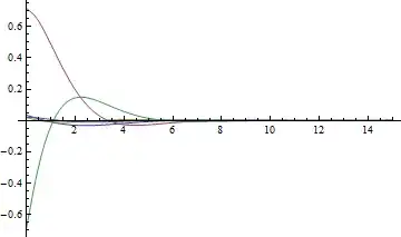
If one runs the integration on from the results with inf = 9 then one can see that the second derivative was made to pass through the point 9 but is not zero subsequently. Here I have run the inf = 9 case to get the roots but now solve and plot using these values for inf = 15.

inf = 15;
sol = First@NDSolve[Evaluate[Join[eqns, ic0,
       {(a[0]'')[0] == 
         a0, (a[1]'')[0] == 
         a1, (b[1]'')[0] == b1,
        (a[2]'')[0] == 
         a2, (b[2]'')[0] == b2}] /. 
      Join[{α -> 0.1}, rts]],
    {a[0], a[1], b[1], a[2], b[2], a[0]'', a[1]'', b[1]'', a[2]'', 
     b[2]''}, {η, 0, inf}];
Join[{Plot[Evaluate[{a[0]''[η]} /. sol], {η, 0, inf}, 
   PlotRange -> All]},
 Table[
  Plot[Evaluate[{a[n]''[η], b[n]''[η]} /. sol], {η, 0, 
    inf}, PlotRange -> All],
  {n, 1, 2}
  ]
 ]

So I have failed to get the asymptotic solution. I have tried integrating over an interval at large values of η and then using FindMinimum but this does not give good results.

Do you have any further ideas? Thanks

Answer 1

Once again, let's turn to the primitive finite difference method (FDM). I'll use pdetoae for the generation of difference equation:

var = Flatten@{a /@ Range[0, 2], b /@ Range@2}
bc = D[Through@var[t] == 0 // Thread, t, t] /. t -> inf

inf = 15;
points = 200;
difforder = 4;
grid = Array[# &, points, {0, inf}];
ptoafunc = pdetoae[var[η], grid, difforder];
del = #[[3 ;; -2]] &;
ae = del /@ ptoafunc@eqns;
(* Definition of pdetoae isn't included in this post,
   please find it in the link above. *)
aebc = ptoafunc@{ic0, bc};

sollst = Partition[
    With[{guess = 1}, 
      FindRoot[{ae, aebc} /. {α -> 1/10}, 
       Flatten[Table[{var[[i]][η], guess}, {i, 5}, {η, grid}], 1]]][[All, -1]],
     points]; // AbsoluteTiming

Remark

The following way to calculate sollst doesn't require one to use del:

fullsys = Flatten@ptoafunc@{eqns, ic0, bc};

lSSolve[obj_List, constr___, x_, opt : OptionsPattern[FindMinimum]] := 
 FindMinimum[{1/2 obj^2 // Total, constr}, x, opt]
lSSolve[obj_, rest__] := lSSolve[{obj}, rest]

sollst = Partition[
    With[{guess = 1}, 
      lSSolve[Subtract @@@ fullsys /. {α -> 1/10}, 
       Flatten[Table[{var[[i]][η], guess}, {i, 5}, {η, grid}], 1]]][[2, 
      All, -1]], points]; // AbsoluteTiming

But notice it's slower and less robut compared to the FindRoot approach.

solfunclst = ListInterpolation[#, grid] & /@ sollst;

Plot[D[Through@solfunclst[x], x, x] // Evaluate, {x, 0, inf}, PlotRange -> All]

FindRoot still spits out lstol, but further check by adjusting points, difforder, etc. shows the result seems to be accurate enough.