plotting solutions of the Schrödinger equation for the hydrogen atom

Question

I'm not very familiar with coding in Mathematica but I'd like to plot the solutions (actually Spherical Harmonic orbital solutions) of the Schrödinger equation for the hydrogen atom. To be more precise, it would be grate if you could help me reproduce some plots of this picture.

Since the only function I know of to do something like that is SphericalPlot3D I tried the following

SphericalPlot3D[
  Abs[SphericalHarmonicY[0, 0, r, w]]^2, {r, 0, Pi}, {w, 0, 2 Pi}, 
  Boxed -> True, Axes -> True, PlotPoints -> 250, Mesh -> 4]

This already looked quite nice but I had some trouble adjusting the length of the axis to fit the whole plot (is there a way to let Mathematica do that automatically). I also couldn't reproduce the ColorFunction used in the picture above (1). Another thing is that I don't know how to do is cut off a piece of the plot (to see what's "inside").

Thanks for the help in advance, Sito.

You should be careful with the plots in the figure referenced as they are the wave functions of the Hydrogen atom and NOT the spherical harmonics only. You must also include in your SphericalPlot3D the radial functions. — José Antonio Díaz Navas, Dec 01 '17 at 11:16
@JoséAntonioDíazNavas The problem is, when I try to do that I get a error... I found something on the net for a two-dimensional density plot link but I don't know how to transfer that to a 3D-Spherical Plot. — Sito, Dec 01 '17 at 12:35

score 3 · Accepted Answer · edited Dec 01 '17 at 20:23

I heve detected some errors in the equations you provided in the image link. In addition, and after viewing the plots you want to reproduce, I have to say that the modulus square of wave functions gives probability density in the context of Quantum Mechanics. Therefore, I have tried the following correct expression in spherical coordinates, and then I have transformed to cartesians:

 a0 = Quantity["BohrRadius"]/Quantity["Meters"];

 ψ[{n_, l_, m_}, {r_, θ_, ϕ_}] := With[
   {ρ = 2 r/(n a0)}
 , Sqrt[(2/(n a0))^3 (n - l - 1)!/(2 n (n + l)!)]
   Exp[-ρ/2] ρ^l LaguerreL[n - l - 1, 2 l + 1, ρ] 
   SphericalHarmonicY[l, m, θ, ϕ]
 ];

 f = TransformedField[
   "Spherical" -> "Cartesian", ψ[{n, l, m}, {r, θ, ϕ}]
 , {r, θ, ϕ} -> {x, y, z}
];

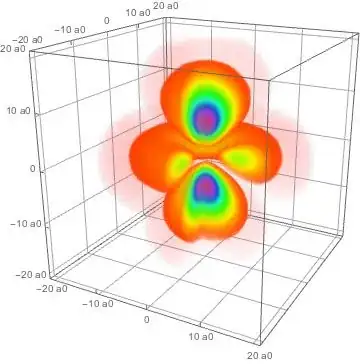
Now I have used DensityPlot3D more appropriate to show probability density, so for $\psi(5,2,1,r,\theta,\phi)$, I obtained:

where the axes are in Bohr radius units.

The problem I found is that the scale must be controlled. Of course, the colours should be managed accordingly to the best visualisation. Another example with ColorFunction->Hue and $\psi(3,2,0,r,\theta,\phi)$

DensityPlot3D[(Abs@f)^2, {x, -20 a0, 20 a0}, {y, -20 a0, 
20 a0}, {z, -20 a0, 20 a0}, 
RegionFunction -> Function[{x, y, z}, x < 0 || y > 0], 
ColorFunction -> Hue, ColorFunctionScaling -> True, 
ViewPoint -> {1.3, -2.4, 1.}, 
FaceGrids -> {{-1, 0, 0}, {0, 1, 0}, {0, 0, -1}}, 
Ticks -> Table[{{-20 a0, "-20 a0"}, {-10 a0, "-10 a0"}, {0, 
 "0"}, {10 a0, "10 a0"}, {20 a0, "20 a0"}}, {i, 3}]]

I think that you can make a piramidal table taking into account the other answer.

Hope this helps.

First of all, thanks for the solution to my problem! If there were some errors in the functions (pictures) I'm sorry, I didn't notice them.
For me personally it makes more sense to do a denisity plot (just from Quantum mechanics point of view ) but, just out of curiosity, what is shown in the picture I referenced in my first post? And how would I realize something like that? — Sito, Dec 01 '17 at 20:01
You are welcome. I think those plots are the wavefunctions at a given probability value. They were plotted posibly by means of ContourPlot3D. However, be advised you need to know these density values for the contours. In my humble opinion, that shows a partial information. We have now more powerful tools to provide the whole picture. — José Antonio Díaz Navas, Dec 01 '17 at 20:50

David G. Stork · Answer 2 · 2017-12-01T00:38:39.477

Try:

 Column[
     Table[
     SphericalPlot3D[
      Abs[SphericalHarmonicY[n, m, φ, θ]]^2,
      {φ, 0, π}, {θ, 0, 3 π/2},
      Boxed -> True,
      Axes -> True,
      PlotPoints -> 250,
      Mesh -> 4,
      PlotRange -> All,
      ColorFunction -> "TemperatureMap",
      PlotStyle -> Automatic],
     {n, 1, 3},
     {m, -n, n, 2}],
     Center]

"Cutting away" merely means you plot {θ, 0, 3 π/2}, not the full range {θ, 0, 2 π}.

plotting solutions of the Schrödinger equation for the hydrogen atom

2 Answers2