I am struggling with writing a stochastic version of Lotka-Volterra predator-prey model. This is as far as I have gotten:
a = 0.1;
b = 0.2;
c = 0.3;
d = 0.4;
proc =
RandomFunction[
ItoProcess[
{\[DifferentialD]X[t] == (a \[DifferentialD]t X[t] + \[DifferentialD]W[t]) -
b \[DifferentialD]t X[t] Y[t],
\[DifferentialD]Y[t] == -c \[DifferentialD]t Y[t] +
d \[DifferentialD]t Y[t] X[t]},
{X[t], Y[t]}, {{X, Y}, {0.2, 0.2}}, t,
W \[Distributed] WienerProcess[0, 0.1]], {0, 100, 0.01},
Method -> "StochasticRungeKuttaScalarNoise"];
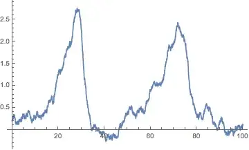
ListLinePlot[proc, PlotRange -> All]
For some reason, only one variable depends on the stochastic noise and it does not bear influence on the other part of the equation, I have tried to correct it, but no matter what I do, no luck.
First thing would be to get it working correctly, then I would worry about excluding "extinction Values > 0", since we are not interested in those.
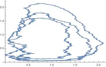
Also, in regards to the graph, is there other way I would create a phase plot (X against Y)? My current way:
ListLinePlot[proc["Values"], PlotRange -> All]
plots X and Y, against time. How would I plot only X in time?
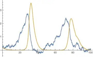

ListLinePlot[Transpose@proc["Values"], PlotRange -> All]– m_goldberg Jan 20 '18 at 07:12