underlying data for `QuantilePlot[]`

Question

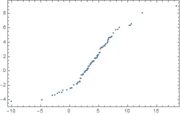
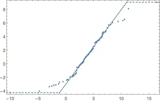
What is the best way to produce the actual pairs of points shown by QuantilePlot? Would anyone have an implementation? (I am interested in the simplest possible version: QuantilePlot[l1, l2], where l1, l2 are lists of numbers.

See https://mathematica.stackexchange.com/questions/19859/plot-extract-data-to-a-file — Vsevolod A., Mar 15 '18 at 19:32
And https://stackoverflow.com/questions/18921651/get-points-of-listplot-in-mathematica — Vsevolod A., Mar 15 '18 at 19:34
@VsevolodA. Yes, I am aware that foo[[1, 2, 2, 2, 3, 1]] works, but that is not the real question, since I have no idea what parameters mathematica uses (number of points, etc). I can guess, but this is not very satisfying. — Igor Rivin, Mar 15 '18 at 19:37
Read your question again: "What is the best way to produce the actual pairs of points shown by QuantilePlot". — Vsevolod A., Mar 15 '18 at 20:04
@Vsevolod, that's still not the best way, then; gwr's answer gives a direct method to produce the points from scratch, without the processing overhead of QuantilePlot[]. — J. M.'s missing motivation, Mar 16 '18 at 12:17

gwr · Accepted Answer · 2018-03-16T10:45:05.813

Reverse-Engineering Mathematica's Q-Q-Plots

You can also use Quantile directly which gives more control about what is happening and precision maybe:

Inspecting points produced by Bob Hanlon's approach and playing around with other sample sizes reveals that Mathematica appears to use the range specified by $\frac{k-0.3}{n+0.4}$ with $k = 1, \ldots, n$ to produce quantiles. Other possibilities are given by Wikipedia (cf. source no. 10 for the option given here).

Thus:

SeedRandom[0];

data1 = RandomVariate[NormalDistribution[2, 3], 100];
data2 = RandomVariate[StudentTDistribution[4, 2, 3], 200];

pts = With[
    {
        n = Min @@ Length /@ { data1, data2 }        
    },
    Curry[Quantile][ Table[(k - 0.3)/(n + 0.4), {k, n}] ] /@ {data2, data1} // Transpose
    (* or Map[ Quantile[#, Table[ ... ]]&] @ {data2,data1} // Transpose *)
];

ListPlot[ pts, Axes-> False, Frame -> True ]

We can compare with the QuantilePlot points using Bob Hanlon's approach:

pts2 = Cases[plot, Point[pts_] :> pts, Infinity][[1]];
pts2 - pts

{{0.,0.}, ... , {0.,0.}}

This comparison also holds for samples sizes 200, 300 that I tested so far.

Thanks, Sjoerd C. de Vries, for pointing out the more general range-regime for Q-Q-Plots.

Nice use of the new 11.3 function Curry . The Range call, though, is only correct because data 1 happens to be 100 points long. It doesn't generalize to differently sized data sets. — Sjoerd C. de Vries, Mar 15 '18 at 22:16
Ah, you beat me to it. To add: the positioning method is due to Bernard and Bos-Levenbach (English version). Spelunking confirms that this method is used internally by the helper function System`QuantilePlotDump`plottingPosition[]. — J. M.'s missing motivation, Mar 16 '18 at 12:15
In the case where one is comparing against a distribution instead of another dataset, EstimatedDistribution[] is used on the data (NormalDistribution[] is the default distribution to compare against), and then this is used in the computation of the second set of quantiles. — J. M.'s missing motivation, Mar 16 '18 at 12:19

score 1 · Answer 2 · answered Mar 15 '18 at 19:54

SeedRandom[0];

data1 = RandomVariate[NormalDistribution[2, 3], 100];
data2 = RandomVariate[StudentTDistribution[4, 2, 3], 200];

plt = QuantilePlot[data1, data2]

Use Cases to extract the points

pts = Cases[plt, Point[pts_] :> pts, Infinity][[1]];

Dimensions[pts]

{100, 2}

In this case there are 100 points.

ListPlot[pts, Frame -> True, Axes -> False]

underlying data for `QuantilePlot[]`

2 Answers2