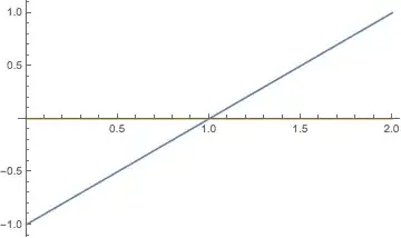
Most minimal approach: just solve for equilibria and plot. I'll set a=1 and plot x vs b.
eq = Solve[{0 == x (y - 1), 0 == -y (x + a) + b}, {x, y}]
(* {{x -> -a + b, y -> 1}, {x -> 0, y -> b/a}} *)

a = 1;
Plot[Evaluate[x /. eq], {b, -0, 2}]
Now, maybe you want to know which branch is stable. We can do this analytically by finding eigenvalues of the Jacobian matrix, evaluated at the two equilibria.
j = D[{x (y - 1), -y (x + a) + b}, {{x, y}}]
(* {{-1 + y, x}, {-y, -1 - x}} *)

Eigenvalues[j /. eq[[1]]]
(* {-1, 1 - b} *)
This (blue) equilibrium is stable when 1-b<0, equivalently when b>1.
Eigenvalues[j /. eq[[2]]]
(* {-1, -1 + b} *)
This (golden) equilibrium is stable when -1+b<0, equivalently when b<1. Therefore there is an exchange of stability at the transcritical bifurcation point b==1.
Finally, maybe you want to style the equilibria in the bifurcation diagram to show their stability (say, solid=stable and dashed=unstable). First, define the dominant eigenvalue
λ[bval_?NumericQ, pt_] := Max[Re[Eigenvalues[j /. pt] /. b -> bval]];
Then plot each equilibrium using MeshFunctions to indicate the stability.
Show[
  Plot[x /. eq[[1]], {b, 0, 2}, MeshStyle -> None,
    MeshFunctions -> {λ[#1, eq[[1]]] &}, Mesh -> {{0}},
    MeshShading -> {Directive[Black, Thick], Directive[Black, Dashed]}],
  Plot[x /. eq[[2]], {b, 0, 2}, MeshStyle -> None,
    MeshFunctions -> {λ[#1, eq[[2]]] &}, Mesh -> {{0}},
    MeshShading -> {Directive[Black, Thick], Directive[Black, Dashed]}]
]
