2

I have the following differential equation

m*x''[t] + k*x'[t] - randomForce[t] == 0

which describes an oscillating particle with mass m, moving in a medium with friction coefficient k and excited by a random white noise force randomForce.

As I understand from the documentation (guide/StochasticDifferentialEquationProcesses) instead of solving the differential equation I could also use e.g. the corresponding OrnsteinUhlenbeckProcess.

In my case are: m = 6.137*10^-10; (* in g *); k = 9.2055*10^-10; (* in g/s *).

How can the OrnsteinUhlenbeckProcess be used to solve the upper differential equation?

Please see also the related question.
mrz
  • 11,686
  • 2
  • 25
  • 81

1 Answers1

6

One could do:

k = 9.2055*10^-10;
m = 6.137*10^-10;

proc[x0_, v0_, γ_, f_] = ItoProcess[
     {\[DifferentialD]x[t] == v[t] \[DifferentialD]t, 
      \[DifferentialD]v[t] == -γ v[t] \[DifferentialD]t + f \[DifferentialD]w[t]}, 
     {x[t], v[t]}, {{x, v}, {x0, v0}}, t,  w \[Distributed] WienerProcess[]]

Then one can calculate properties:

Mean[proc[x0, v0, γ, f][t]]
(* {(v0 - E^(-t γ) v0 + x0 γ)/γ, E^(-t γ) v0} *)

or do simulations:

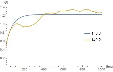
sims0 = RandomFunction[proc[0.5, 1.1,  k/m, 0.0], {0., 10., 0.01}]
sims = RandomFunction[proc[0.5, 1.1,  k/m, 0.2], {0., 10., 0.01}]

ListLinePlot[{sims0["ValueList"][[1, All, 1]], sims["ValueList"][[1, All, 1]]}, 
 PlotLegends -> Placed[{"f=0.0", "f=0.2"}, {Right, Center}], AxesLabel -> {"time", "x[t]"}]

enter image description here

b.gates.you.know.what
  • 20,103
  • 2
  • 43
  • 84
  • Thank you for your help ... I do not understand why x is saturating, that should not be the case for the given differential equation (there is no confining potential). – mrz Apr 10 '18 at 12:55
  • 2
    See if you agree with Simplify[Limit[Mean[proc[x0, v0, \[Gamma], f][t]], t -> Infinity], Assumptions -> {\[Gamma] > 0, (x0 | v0) \[Element] Reals}]. – b.gates.you.know.what Apr 10 '18 at 13:21
  • Yes correct, I agree. When I use the parameters drift and volatility in WienerProcess then it looks to me more “real”, like what I see in experiments. I have to play around with these two parameters. – mrz Apr 10 '18 at 15:13
  • How would you extend this solution to obtain the movement in 2d? Is this correct: sims=RandomFunction[proc[0.5, 1.1, k/m, 1], {0.1, 10., 0.1}, 2]and then ListLinePlot[sims[[2, 1, 1]], AspectRatio -> Automatic] – mrz Apr 10 '18 at 15:42
  • 1
    You would need to define the 2d equations of motion along the same lines (and decide whether the forces are correlated, ...). – b.gates.you.know.what Apr 10 '18 at 15:59