Investigating mesh suitability

Question

Trying to get a good mesh often requires significant work. For the finite element package we can have first and second order elements. Thus this suggests we need fine good quality meshes rather than rely on high order shape functions. If you have a point of interest that requires a fine mesh size how quickly can the mesh size change as you move away from this point? Are there tools for this? This question looks at the overal quality of the mesh. Here I am interested in the quality around a point of interest.

To be specific my current problems with stress occur on the boundaries. I note that if I put in a small mesh length at the boundary it will be nicely expanded into the interior.

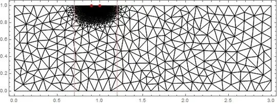
Here is an example in which I have two points on the boundary where I want a fine mesh.

    Needs["NDSolve`FEM`"];
L = 3;  (* Length *)
h = 1;  (* Height *)
Y = 10^3;  (* Modulus of elasticity *)
ν = 33/100;  (* Poisson ratio *)
gLS = h/5;   (* Basic grid length scale *)
sgLS = gLS/200;   (* Small grid length scale *)
p1 = L/3; p2 = 1.337;  (* Points of interest *)
nn = 4;
cc = {{0, 0}, 
   Sequence @@ Table[{p2 + n sgLS, 0}, {n, -nn, nn}], {L, 0}, {L, h}, 
   Sequence @@ Table[{p1 + n sgLS, h}, {n, -nn, nn}], {0, h}};
ccp = Partition[Range[Length@cc], 2, 1, 1];
bmesh = ToBoundaryMesh["Coordinates" -> cc, 
   "BoundaryElements" -> {LineElement[ccp]}];
mesh = ToElementMesh[bmesh, MaxCellMeasure -> {"Length" -> gLS}];
Show[mesh["Wireframe"], 
 Graphics[{Red, PointSize[0.01], Point[{{p1, h}, {p2, 0}}], 
   Thickness[0.01], Line[{{p2 - gLS/2, h/2}, {p2 + gLS/2, h/2}}]}]]

Mathematica graphics

The red line has a length that is my requested basic mesh length scale and I estimate that the actual mesh length scale is about 75% of this which is good. Can the actual grid length scale in an area be extracted. I have also put in 5 closely spaced points on the boundary where I need good resolution. This has been done and the mesh size has been automatically expanded away from these points. A zoom shows this.

d = 0.02;
Show[mesh["Wireframe"], 
 Graphics[{Red, PointSize[0.02], Point[{{p1, h}, {p2, 0}}] }], 
 Frame -> True, PlotRange -> {{p2 - d, p2 + d}, {0, 2 d}}]

Mathematica graphics

How do I determine if this rate of mesh expansion away from the point of interest is good enough for my application? What is the heuristic used in making this mesh? Can it be controlled? Of course I can go to a MeshRefinementFunction but how quickly should I expand that if I use it?

The answer to the appropriate rate of expansion probably depends on the problem and the fact that we have second order elements. So here are some modules to run a problem.

planeStress[
  Y_, ν_] := {Inactive[
     Div][({{0, -((Y ν)/(1 - ν^2))}, {-((Y (1 - ν))/(2 (1 \
- ν^2))), 0}}.Inactive[Grad][v[x, y], {x, y}]), {x, y}] + 
   Inactive[
     Div][({{-(Y/(1 - ν^2)), 
        0}, {0, -((Y (1 - ν))/(2 (1 - ν^2)))}}.Inactive[Grad][
       u[x, y], {x, y}]), {x, y}], 
  Inactive[Div][({{0, -((Y (1 - ν))/(2 (1 - ν^2)))}, {-((Y \
ν)/(1 - ν^2)), 0}}.Inactive[Grad][u[x, y], {x, y}]), {x, y}] +
    Inactive[
     Div][({{-((Y (1 - ν))/(2 (1 - ν^2))), 
        0}, {0, -(Y/(1 - ν^2))}}.Inactive[Grad][
       v[x, y], {x, y}]), {x, y}]}

ClearAll[stress2D]
stress2D[{uif_InterpolatingFunction, 
   vif_InterpolatingFunction}, {Y_, ν_}] :=
 Block[{fac, dd, df, mesh, coords, dv, ux, uy, vx, vy, ex, ey, gxy, 
   sxx, syy, sxy}, dd = Outer[(D[#1[x, y], #2]) &, {uif, vif}, {x, y}];
  fac = Y/(1 - ν^2)*{{1, ν, 0}, {ν, 1, 0}, {0, 
      0, (1 - ν)/2}};
  df = Table[Function[{x, y}, Evaluate[dd[[i, j]]]], {i, 2}, {j, 2}];
  (*the coordinates from the ElementMesh*)
  mesh = uif["Coordinates"][[1]];
  coords = mesh["Coordinates"];
  dv = Table[df[[i, j]] @@@ coords, {i, 2}, {j, 2}];
  ux = dv[[1, 1]];
  uy = dv[[1, 2]];
  vx = dv[[2, 1]];
  vy = dv[[2, 2]];
  ex = ux;
  ey = vy;
  gxy = (uy + vx);
  sxx = fac[[1, 1]]*ex + fac[[1, 2]]*ey;
  syy = fac[[2, 1]]*ex + fac[[2, 2]]*ey;
  sxy = fac[[3, 3]]*gxy;
  {ElementMeshInterpolation[{mesh}, sxx],
   ElementMeshInterpolation[{mesh}, syy],
   ElementMeshInterpolation[{mesh}, sxy]
   }]

The example problem (a MWE) is

{uif, vif} = 
  NDSolveValue[{planeStress[Y, ν] == {0, 
      NeumannValue[-1, 0 <= x <= p1 && y == h]}, 
    DirichletCondition[v[x, y] == 0, 0 <= x <= p2 && y == 0], 
    DirichletCondition[u[x, y] == 0, x == 0 && y == 0]}, {u, 
    v}, {x, y} ∈ mesh];
{σxx, σyy, σxy} = 
  stress2D[{uif, vif}, {Y, ν}];
Plot[{σxx[x, 0], σyy[x, 0], 500 vif[x, 0]}, {x, 0, L}, 
 PlotRange -> All, Frame -> True, Axes -> False, 
 PlotLegends -> 
  LineLegend[{"\!\(\*SubscriptBox[\(σ\), \(xx\)]\)", 
    "\!\(\*SubscriptBox[\(σ\), \(yy\)]\)", "500 v"}]]

Mathematica graphics

As you can see the results look nice and have a singularity where I have put my point (which is correct). However, is my mesh adequate? How can I tell? Is there a rule of thumb?

Thanks for any advice.

If you specify "MeshOrder"->1 to ToElementMesh you will get a first order mesh and not a second order mesh. So you can have either or. — user21, Apr 24 '18 at 13:26
@user21 Good point. I am assuming that second order is better particularly as I have to take derivatives of the solution to find stresses. Are you suggesting that a first order mesh with twice the number of elements could be a better approach? — Hugh, Apr 24 '18 at 13:29
Hugh, just as a remark: The error of the discrete solution does also depend on the smoothness of the true solution, i.e. the solution of the continuous problem. For example, second order finite elements are only better than first order solutions on the same mesh in the $H^1$-sense if the true solution has regularity better than $H^2$. So if the true solution is expected to have low regularity, first order elements might perform as well (or better due to their smaller stencils) than second order elements. — Henrik Schumacher, Apr 24 '18 at 22:27
@Hugh, no I am not suggesting that. I am just saying that what you state in your pose (that you can only have second order meshes) is not correct. You could update that. — user21, Apr 25 '18 at 07:09
From what I understand from your question what you want to do is a proper convergence analysis. Take a problem for which you have a solution and measure the approximation quality for successively refined meshes. Basically a manual adaptive mesh refinement. — user21, Apr 25 '18 at 07:11
@user21 I have corrected the point about mesh order. The suggestion of a convergence analysis seems the correct approach. Is there an example of how to do this somewhere? The example problem above has no know solution. Should I just look at the errors as the mesh is refined? — Hugh, Apr 25 '18 at 09:28
@HenrikSchumacher Thanks for your remark. I have been pondering this. As we calculate displacements but require stresses (which are derivatives of displacements) do we always have to have a second order mesh? I am not clear what the derivative does with a first order mesh. Do you know how to investigate this? — Hugh, Apr 25 '18 at 09:34
That's a delicate question. Classical convergence proofs for FEM are performed in the energy space of the PDE, that is the space where the weak formulation of the PDE is well-defined and coercive. For elliptic second order PDE, this is $H^1=W^{1,2}$, the space of $L^2$ functions with a weak derivative in $L^2$. That is a pretty weak norm: For instance, a $W^{1,2}$ function on a domain of dimension greater or equal to 2 need not be continuous... — Henrik Schumacher, Apr 25 '18 at 09:44
@Hugh In the [tag:acegen] documentation there is an example of adaptive mesh refinement (of ElementMesh) with extensive explanation. Maybe some sections could be useful for your case? — Pinti, Apr 25 '18 at 09:49
But there are also $L^\infty$-error estimates (which is in fact $C^0$-estimates) in the literature. That means that pointwise evaluations of the discrete solutions can be trusted (up to a certain mesh-dependent error). But one should be cautious with pointwise evaluations of first derivatives: The rigorous error estimates that I know can only estimate the $L^2$ error of first derivatives. — Henrik Schumacher, Apr 25 '18 at 09:50
That means that you should trust the computed stresses only in average over relatively large domains (large compared to the mesh cells). I am quite sure that also the $L^\infty$-error of discrete solutions should be controllable if the true solution and the boundary of the domain are sufficiently well-behaved. But I just don't know any rigorous proof for that in the literature. — Henrik Schumacher, Apr 25 '18 at 09:52
@Pinti Thanks I had a look but none of the many postings seemed to mention adaptive mesh refinement. Please could you be more specific? — Hugh, Apr 25 '18 at 10:57
@HenrikSchumacher Thanks for the comments. It is good to know that there is some deep understanding of the issues. Is there a practical way of looking at errors? Do I just do lots of cases and look at differences? If so how do I know the errors are getting better as I refine the mesh? — Hugh, Apr 25 '18 at 11:00
As a rule of thump: Let $h$ be the maximal diameter of the mesh cells and assume that the aspect ratios of all mesh cells is confined to a neighborhood of 1 and assume that the true solution has sufficient regularity. Then first order FE should have $L^2$-error proportional to $h^2$ and $H^1$-error proportional to $h$ (if the true solutions has regularity $H^2$. I think, second order FE should have $L^2$-error proportional to $h^3$ and $H^1$-error proportional to $h^2$ (if the true solution is in $H^3$). There are also localized version of theses statements. — Henrik Schumacher, Apr 25 '18 at 11:10
For adaptive finite elements, there are also ways to estimate the errors a posteriori from the already computed discrete solution without knowing the true solution. "a posteriori error estimates" along with "adaptive FEM" should make good buzzwords for google queries. — Henrik Schumacher, Apr 25 '18 at 11:11
In practice, people do exactly what you proposed: Test various mesh configurations with problems of known true solution that are somewhat similar to the problem you want to solve in the end. This $h^k$ calculus can give you some intuition how the errors should behave if the mesh is refined. The purely theoretical results are all quite nice but in the end they boil down to "the more you butter the tastier the sandwich"... — Henrik Schumacher, Apr 25 '18 at 11:24
@Hugh I meant the documentation of the AceFEM package (you can install free trial version). The example has been added in version 6.822 and you can find it if you search for "adaptive mesh refinement" in Mathematica help centre. — Pinti, Apr 25 '18 at 12:31
@HenrikSchumacher Following your suggestions I have had a go at looking at convergence. I have posted this attempt as an answer. Is this along the lines of your comments? — Hugh, Apr 25 '18 at 17:40

score 2 · Answer 1 · answered Apr 25 '18 at 17:38

This is not an answer but following suggestions from the comments I am having a go at doing a convergence analysis. Henrik Schumacher has given guidance on what should happen and I am keen to have a go.

I have made the problem an attempt to see if one can make a good loading for the block being stressed. I looked at putting on a rectangular loading here but I have come to the conclusion that this is not possible. Instead I will put a tapered loading onto the block.

Here are the parameters and function to produce a loading that is constant and then taperes to zero (illustrated below).

Y = 10^3;  (* Modulus of elasticity *)
ν = 33/100;  (* Poisson ratio *)
L = 3;  (* Length *)
h = 1;  (* Height *)
p1 = L/3 - h/10;(* start of taper *)
p2 = L/3; (* end of taper *)
gLS = h/5.; (* grid length scale *)

ClearAll[force];
force[x_, {p1_, p2_}] := 
 Piecewise[{{-1, 0 <= x <= p1}, {-1 + (x - p1)/(p2 - p1), 
    p1 < x <= p2}}]

By using the modules planeStress and stress2D in the original question the calculation is straightforward. After the calculation I plot the mesh, the target loading and the calculated loading and then the difference between the two to get an error. I am just looking at the stress along the top of the block which should agree with my applied loading.

cc = {{0, 0}, {L, 0}, {L, h}, {p2, h}, {p1, h}, {0, h}};
bp = Partition[Range@Length@cc, 2, 1, 1];
bmesh = ToBoundaryMesh["Coordinates" -> cc, 
   "BoundaryElements" -> {LineElement[bp]}];
mesh = ToElementMesh[bmesh, MaxCellMeasure -> {"Length" -> gLS}];
{uif, vif} = 
  NDSolveValue[{planeStress[Y, ν] == {0, 
      NeumannValue[force[x, {p1, p2}], 0 <= x <= p2 && y == h]},
    DirichletCondition[v[x, y] == 0, 0 <= x <= L && y == 0],
    DirichletCondition[u[x, y] == 0, x == 0 && y == 0]}, {u, 
    v}, {x, y} ∈ mesh];
{σxx, σyy, σxy} = 
  stress2D[{uif, vif}, {Y, ν}];
mesh["Wireframe"]
Plot[{force[x, {p1, p2}], σyy[x, h]}, {x, p1 - gLS, p2 + gLS}, 
 Frame -> True, FrameLabel -> {"x", "Stress"}, 
 PlotLegends -> LineLegend[{"Target", "Calculated"}]]
Plot[{force[x, {p1, p2}] - σyy[x, h]}, {x, p1 - gLS, p2 + gLS},
  Frame -> True, FrameLabel -> {"x", "Error"}, PlotRange -> All]

Mathematica graphics

As can be seen the error is quite large (about 12%). The objective is to refine the grid and hence reduce the error. The function I am going to use to refine to grid is as follows

$$\text{area}=\frac{1}{4} \sqrt{3} \left(e r+r_0\right){}^2 $$

Here area is the area of the element and $r$ is the distance from the point I am concerned about (here p1 and p2). $r_0$ is the smallest element "diameter" and $e$ is the rate of expansion (must be less than 1). Thus the element "diameter" will be expanded linearly from $r_0$ to a maximum size I also have to specify. I will make the maximum size the grid length scale I have defined.

So now I need to check convergence with different smallest "diameters" and different rates of expansions. Here are a couple of modules that solve with differing values of $r_0$ and $e$.

ClearAll[meshSolve];
meshSolve[r0_, e_] := 
 Module[{cc, bp, bmesh, mesh, uif, 
   vif, σxx, σyy, σxy},
  cf = Compile[{{c, _Real, 2}, {a, _Real, 0}},
    Block[{r, com, c1 = {p1, h}, c2 = {p2, h}},
     com = Total[c]/3;
     r = Min[{Norm[com - c1], Norm[com - c2]}];
     If[r < gLS && a > Sqrt[3]/4 (r0 + e r)^2, True, False]
     ]
    ];
  cc = {{0, 0}, {L, 0}, {L, h}, {p2, h}, {p1, h}, {0, h}};
  bp = Partition[Range@Length@cc, 2, 1, 1];
  bmesh = 
   ToBoundaryMesh["Coordinates" -> cc, 
    "BoundaryElements" -> {LineElement[bp]}];
  mesh = ToElementMesh[bmesh, MaxCellMeasure -> {"Length" -> gLS}, 
    MeshRefinementFunction -> cf];
  {uif, vif} = 
   NDSolveValue[{planeStress[Y, ν] == {0, 
       NeumannValue[force[x, {p1, p2}], 0 <= x <= p2 && y == h]},
     DirichletCondition[v[x, y] == 0, 0 <= x <= L && y == 0],
     DirichletCondition[u[x, y] == 0, x == 0 && y == 0]}, {u, 
     v}, {x, y} ∈ mesh];
  {σxx, σyy, σxy} = 
   stress2D[{uif, vif}, {Y, ν}];
  {uif, vif, σxx, σyy, σxy}
  ]

ClearAll[findErrors];
findErrors[{uif_, vif_, σxx_, σyy_, σxy_}, r0_, 
  e_] := Module[{cc, ee},
  cc = Select[
    uif["Coordinates"][[1]][
     "Coordinates"], #[[2]] == h && p1 - gLS < #[[1]] <= p2 + gLS &];
  ee = {#[[1]], (σyy[#[[1]], #[[2]]] - 
        force[#[[1]], {p1, p2}])} & /@ Sort[cc];
  {r0, e, Max[Abs[ee[[All, 2]]]], RootMeanSquare[ee[[All, 2]]]}
  ]

To start I look at different values of $r_0$ keeping $e$ fixed at 0.2.

Timing[errors = Table[
    e = 0.2;
    res = meshSolve[r0, e];
    ee = findErrors[res, r0, e];
    ee,
    {r0, gLS {0.2, 0.1, 0.05, 0.02, 0.01, 0.005, 0.002, 0.001}}];]

This takes about 2 seconds on my machine. The following code tabulates the results and plots them.

TableForm[errors, 
 TableHeadings -> {None, {"\!\(\*SubscriptBox[\(r\), \(0\)]\)", "e", 
    "Maximum error", "RMS error"}}]
ListLogLogPlot[errors[[All, {1, 4}]], Frame -> True, 
 FrameLabel -> {"\!\(\*SubscriptBox[\(r\), \(0\)]\)", "RMS error"}]
ListLogLogPlot[errors[[All, {1, 3}]], Frame -> True, 
 FrameLabel -> {"\!\(\*SubscriptBox[\(r\), \(0\)]\)", "Max error"}]
Plot[{force[x, {p1, p2}] - res[[4]][x, h]}, {x, p1 - gLS, p2 + gLS}, 
 Frame -> True, FrameLabel -> {"x", "Error"}, PlotRange -> All]
mesh = res[[1]]["Coordinates"][[1]];
Show[mesh["Wireframe"],
 Graphics[{Red, PointSize[0.01], Point[{p1, h}], Point[{p2, h}], Pink,
    InfiniteLine[{p1 - gLS, 0}, {0, 1}], 
   InfiniteLine[{p2 + gLS, 0}, {0, 1}]}],
 Frame -> True]

Mathematica graphics

The first two plots are RMS error and maximum error for values of $r_0$. Then for the finest refinement I show the actual error as a function of position and the mesh. In the first plot the errors seem to be going as $ r_0^2$ (except for the smallest two points) which I think is what Henrik Schumacher was suggesting. The failure for the last few points may be due to the fact that I am picking up errors from the edge of the region where I am refining (see the plot of the actual error).

I now explore the effect of the rate of expansion keeping the smallest element size the same.

Timing[errors = Table[
    r0 = 0.001;
    res = meshSolve[r0, e];
    ee = findErrors[res, r0, e];
    ee,
    {e, {0.5, 0.3, 0.2, 0.1}}];]

The plots of the results are now

TableForm[errors, 
 TableHeadings -> {None, {"\!\(\*SubscriptBox[\(r\), \(0\)]\)", "e", 
    "Maximum error", "RMS error"}}]
ListLogLogPlot[errors[[All, {2, 4}]], Frame -> True, 
 FrameLabel -> {"\!\(\*SubscriptBox[\(r\), \(0\)]\)", "RMS error"}]
ListLogLogPlot[errors[[All, {2, 3}]], Frame -> True, 
 FrameLabel -> {"\!\(\*SubscriptBox[\(r\), \(0\)]\)", "Max error"}]
Plot[{force[x, {p1, p2}] - res[[4]][x, h]}, {x, p1 - gLS, p2 + gLS}, 
 Frame -> True, FrameLabel -> {"x", "Error"}, PlotRange -> All]
mesh = res[[1]]["Coordinates"][[1]];
Show[mesh["Wireframe"],
 Graphics[{Red, PointSize[0.01], Point[{p1, h}], Point[{p2, h}], Pink,
    InfiniteLine[{p1 - gLS, 0}, {0, 1}], 
   InfiniteLine[{p2 + gLS, 0}, {0, 1}]}],
 Frame -> True]

Mathematica graphics

The rms errors seem to go as $e^{1.6}$ is this to be expected? The smaller the rate of expansion the better.

So that what I have discovered is that overall errors seem to go as the grid "diameter" squared and that the smaller the rate of expansion the better.

This seems to give me some confidence in exploring the issue of grid size.

Investigating mesh suitability

1 Answers1