System of equations with sines and cosines

Question

I have a problem with system of equations:

Solve[{x Cos[a] + 52 Cos[a] + 75 Cos[b] + 76 Cos[b - Pi/2] - 75.5 == 0&& 
x Sin[a] + 52 Sin[a] + 75 Sin[b] + Sin[b - Pi/2] == 0 && 
76 Cos[b - Pi/2] + 24.5 + 90 Cos[c] + 56 Cos[d] == 0 && 
76 Sin[b - Pi/2] + 90 Sin[c] + 56 Cos[d] == 0 && 
90 Cos[c] + 84 Cos[d + Pi] + 54 Cos[d + Pi/2] - e == 0 && 
90 Sin[c] + 84 Sin[d + Pi] + 54 Sin[d + Pi/2] - y == 0}, {y, a, b, c, d, e}]

I have to get an results of all variables with parametr x, but computer cannot give me an anwser. What should I do with this?

Do you know any constraints that you could apply to the values of the variables? What do you intend to do with the solutions? Would a numerical approach be viable, considering the next step in your work? — MarcoB, Apr 26 '18 at 22:37
Could try turning it into an algebraic system using method here or here — Daniel Lichtblau, Apr 27 '18 at 15:00

score 3 · Answer 1 · answered Apr 30 '18 at 21:45

You can get an anylytical solution depending on x with the trick, writing Sin[a]->sa and Cos[a]->ca and adding the equation sa^2+ca^2==1.

eqs[x_] = 
 Rationalize[
x Cos[a] + 52 Cos[a] + 75 Cos[b] + 76 Cos[b - Pi/2] - 75.5 == 0 && 
x Sin[a] + 52 Sin[a] + 75 Sin[b] + Sin[b - Pi/2] == 0 && 
76 Cos[b - Pi/2] + 24.5 + 90 Cos[c] + 56 Cos[d] == 0 && 
76 Sin[b - Pi/2] + 90 Sin[c] + 56 Cos[d] == 0 && 
90 Cos[c] + 84 Cos[d + Pi] + 54 Cos[d + Pi/2] - e == 0 && 
90 Sin[c] + 84 Sin[d + Pi] + 54 Sin[d + Pi/2] - y == 0, 0] // 
TrigReduce

eqs2[x_] = (eqs[x] /. {Sin[a] -> sa, Sin[b] -> sb, Sin[c] -> sc, 
   Sin[d] -> sd, Cos[a] -> ca, Cos[b] -> cb, Cos[c] -> cc, 
   Cos[d] -> cd}) && sa^2 + ca^2 == 1 && sb^2 + cb^2 == 1 && 
   sc^2 + cc^2 == 1 && sd^2 + cd^2 == 1 // Simplify;

solx = Solve[eqs2[x] && x > 0, {y, sa, sb, sc, sd, ca, cb, cc, cd, e},
          Reals]

(*   A very large output was generated...   *)

You get root-expressions with conditions for x. In general there are 16 solutions, but not all are valid for given x. Here y is shown for x=20.

Table[y /. N[solx[[j, 1]]] /. x -> 20., {j, 1, 16}]

(*   {Undefined, Undefined, Undefined, Undefined, 111.392, -45.2979, \
      Undefined, Undefined, 91.3868, -23.8247, Undefined, Undefined, \
      Undefined, Undefined, 142.025, -15.8362}   *)

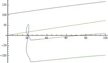
Plotting takes some time

Plot[Evaluate[Table[y /. N[solx[[j, 1]]] /. x -> z, {j, 1, 16}]], {z, 
      0, 100}]

Plot[Evaluate[Table[e /. N[solx[[j, 10]]] /. x -> z, {j, 1, 16}]], {z,
      0, 100}]

Plus or minus ArcSin has to be taken of sa

Plot[Evaluate[
   Table[ArcSin[sa] /. N[solx[[j, 2]]] /. x -> z, {j, 1, 16}]], {z, 0, 
     100}]

score 2 · Answer 2 · answered Apr 26 '18 at 23:48

This seems impossible symbolically, but pretty well behaved numerically.

f[x_] := FindRoot[{x Cos[a] + 52 Cos[a] + 75 Cos[b] + 
  76 Cos[b - Pi/2] - 75.5 == 0 && 
x Sin[a] + 52 Sin[a] + 75 Sin[b] + Sin[b - Pi/2] == 0 && 
76 Cos[b - Pi/2] + 24.5 + 90 Cos[c] + 56 Cos[d] == 0 && 
76 Sin[b - Pi/2] + 90 Sin[c] + 56 Cos[d] == 0 && 
90 Cos[c] + 84 Cos[d + Pi] + 54 Cos[d + Pi/2] - e == 0 && 
90 Sin[c] + 84 Sin[d + Pi] + 54 Sin[d + Pi/2] - y == 
 0}, {{y, -10}, {a, 1}, {b, 1}, {c, 1}, {d, 1}, {e, 50}}]

There are multiple solutions. The choices of initial values here seem to converge on the same branch for x in the interval [0,100]:

Plot[e /. f[x], {x, 0, 100}]

System of equations with sines and cosines

2 Answers2