Maximising a function by finding roots of the derivative is too slow

Question

I have the function r11[t,k] defined as follows

m20[t_, k_] := 
  1/2 (Erf[Sqrt[t]] + 4 t (t + 1) Erfc[Sqrt[t]] - 2 (1 + 2 t) Sqrt[t/Pi] Exp[-t]);
m02[t_, k_] := (1 - Exp[-4 k t])/(2 k);
m11[t_, k_] := (k^2 - k - 1)/k^3 + 
   Sqrt[2 k + 1]/k^3 Erf[Sqrt[t (2 k + 1)]] + 
   2 (k - 1)/k^2 Sqrt[t/Pi] Exp[-(2 k + 1) t] + (1 - k (k - 1) (2 t + 1))/
     k^3 Exp[-2 k t] Erfc[Sqrt[t]] + 
   2/k NIntegrate[(Exp[-(t - s)]/Sqrt[Pi (t - s)] + 
        Erf[Sqrt[t - s]]) (2 Exp[-s] Sqrt[s/Pi] - (2 s + 1) Erfc[Sqrt[s]]) Exp[-2 k s], 
          {s, 0, t}];

 r11[t_, k_] := m11[t, k]/Sqrt[m20[t, k] m02[t, k]];

I want to find its extremum by solving the appropriate equation for some fixed value of time $t=1$.

NSolve[D[r11[1, k], k] == 0, k]

The computation takes long time and doesn't finish at all. Is there a way to speed it up?

Answer 1

To find a local extremum of a function, you could use NMaximize or NMinimize, instead of looking for a root of the derivative. However, the slow-down in numerically solving this problem is coming from repeatedly calling m11[t,k] which needs to numerically integrate on each call.

m20[t_, k_] := 
  1/2 (Erf[Sqrt[t]] + 4 t (t + 1) Erfc[Sqrt[t]] - 
     2 (1 + 2 t) Sqrt[t/Pi] Exp[-t]);
m02[t_, k_] := (1 - Exp[-4 k t])/(2 k);
m11[t_?NumericQ, k_?NumericQ] := (k^2 - k - 1)/k^3 + 
   Sqrt[2 k + 1]/k^3 Erf[Sqrt[t (2 k + 1)]] + 
   2 (k - 1)/k^2 Sqrt[
     t/Pi] Exp[-(2 k + 1) t] + (1 - k (k - 1) (2 t + 1))/
     k^3 Exp[-2 k t] Erfc[Sqrt[t]] + 
   2/k NIntegrate[(Exp[-(t - s)]/Sqrt[Pi (t - s)] + 
        Erf[Sqrt[t - s]]) (2 Exp[-s] Sqrt[s/Pi] - (2 s + 1) Erfc[
          Sqrt[s]]) Exp[-2 k s], {s, 0, t}];
r11[t_, k_] := m11[t, k]/Sqrt[m20[t, k] m02[t, k]];

If you want to search for the root of the derivative, you can use FindRoot

FindRoot[D[r11[1, k], k], {k, 1}] // AbsoluteTiming
(* {14.8238, {k -> 1.15773}} *)

Or you search directly for the maximum

NMaximize[{r11[1, k], k > 0}, k] // AbsoluteTiming
(* {33.5729, {0.95293, {k -> 1.15773}}} *)

You see that in this case, FindRoot is faster, but 14 seconds is still not hyperspeed and the reason is the NIntegrate inside your code. Both results appear to be correct.

Plot[r11[1, k], {k, 0.1, 3}, PlotPoints -> 10, MaxRecursion -> 1, 
 Epilog -> {Line[{{1.1577, 0}, {1.1577, 1}}]}]

Answer 2

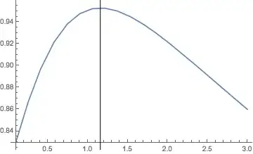
Here's a method to speed things up for you. First, notice that simply restricting the argument patterns of m11 as in the community answer means that the derivative of m11 needs to be computed numerically (which is slow, because the definition of m11 already includes a numerical integration):

Clear[m11]
m11[t_?NumericQ, k_?NumericQ] := (k^2-k-1)/k^3 + Sqrt[2 k+1]/k^3 Erf[Sqrt[t (2 k+1)]] +
    2 (k-1)/k^2 Sqrt[t/Pi] Exp[-(2 k+1) t] +
    (1-k (k-1) (2 t+1))/k^3 Exp[-2 k t] Erfc[Sqrt[t]] + 
    2/k NIntegrate[
        (Exp[-(t-s)]/Sqrt[Pi (t-s)]+Erf[Sqrt[t-s]]) * 
        (2 Exp[-s] Sqrt[s/Pi]-(2 s+1) Erfc[Sqrt[s]]) * Exp[-2 k s],
        {s, 0, t}
    ]

D[m11[1, k], k]

% /. k->1. //AbsoluteTiming

Derivative[0, 1][m11][1, k]

{0.732255, -0.190263}

Instead, let's inactivate the integral in the definition of m11:

Clear[m11]
m11[t_, k_] := (k^2-k-1)/k^3 + Sqrt[2 k+1]/k^3 Erf[Sqrt[t (2 k+1)]] +
    2 (k-1)/k^2 Sqrt[t/Pi] Exp[-(2 k+1) t] +
    (1-k (k-1) (2 t+1))/k^3 Exp[-2 k t] Erfc[Sqrt[t]] + 
    2/k Inactive[NIntegrate][
        (Exp[-(t-s)]/Sqrt[Pi (t-s)]+Erf[Sqrt[t-s]]) * 
        (2 Exp[-s] Sqrt[s/Pi]-(2 s+1) Erfc[Sqrt[s]]) * Exp[-2 k s],
        {s, 0, t}
    ]

Now, the derivative of m11 is a bit more complicated:

dm11 = D[m11[1, k], k]

(-1 + 2 k)/k^3 - (3 (-1 - k + k^2))/k^4 + (2 E^(-1 - 2 k))/( k^3 Sqrt[[Pi]]) - (4 E^(-1 - 2 k) (-1 + k))/(k^3 Sqrt[[Pi]]) + ( 2 E^(-1 - 2 k))/(k^2 Sqrt[[Pi]]) - (4 E^(-1 - 2 k) (-1 + k))/( k^2 Sqrt[[Pi]]) + Erf[Sqrt[1 + 2 k]]/(k^3 Sqrt[1 + 2 k]) - ( 3 Sqrt[1 + 2 k] Erf[Sqrt[1 + 2 k]])/k^4 + ( E^(-2 k) (-3 (-1 + k) - 3 k) Erfc[1])/k^3 - ( 3 E^(-2 k) (1 - 3 (-1 + k) k) Erfc[1])/k^4 - ( 2 E^(-2 k) (1 - 3 (-1 + k) k) Erfc[1])/k^3 - ( 2 Inactive[NIntegrate][ E^(-2 k s) (E^(-1 + s)/(Sqrt[[Pi]] Sqrt[1 - s]) + Erf[Sqrt[1 - s]]) (( 2 E^-s Sqrt[s])/Sqrt[[Pi]] - (1 + 2 s) Erfc[Sqrt[s]]), {s, 0, 1}])/k^2 + ( 2 Inactive[NIntegrate][-2 E^(-2 k s) s (E^(-1 + s)/(Sqrt[[Pi]] Sqrt[1 - s]) + Erf[Sqrt[1 - s]]) (( 2 E^-s Sqrt[s])/Sqrt[[Pi]] - (1 + 2 s) Erfc[Sqrt[s]]), {s, 0, 1}])/k

On the other hand, evaluating the above expression for a numerical value of k only entails a couple numerical integrations. That is, there is no numerical derivative of a function that also includes a numerical integration. So:

Activate[dm11 /. k->1] //AbsoluteTiming

{0.028246, -0.190263}

We get the same result, but it is about 25 times faster. Similarly, we can differentiate r11[t,k] now since the numerical integration is inactive, and define a function to activate the integration after setting the values of the arguments to numerical values:

With[{a1=t_, a2=k_?NumericQ, rhs = D[r11[t,k], k]},
    dr11[a1, a2] := Activate[rhs]
]

The With statement is needed to inject the derivative into the downvalue, but the somewhat obscure a1 and a2 are used to avoid having the patterns automatically modularized. That is, the version without a1 and a2 produces a downvalue like foo[t$_, k$_?NumericQ] := ... instead of foo[t_, k_?NumericQ] := ....

Now, we are ready to use your FindRoot:

FindRoot[foo[1,  k], {k, 1}] //AbsoluteTiming

{0.744606, {k -> 1.15773}}

Quite a bit faster than the version using a pattern restriction with an active NIntegrate.