Just use DSolve in the normal way. No need to use NeumannValue in this case.
pde = D[u[x, t], t] == D[u[x, t], {x, 2}]

DSolve[{pde, Derivative[1, 0][u][1, t] == 0,
  Derivative[1, 0][u][0, t] == 0, u[x, 0] == Sin[Pi x]},
 u[x, t], {x, t}]

(*{{u[x, t] -> 2*Inactive[Sum][((1 + (-1)^K[1])*Cos[Pi*x*K[1]])/
        (E^(Pi^2*t*K[1]^2)*(Pi - Pi*K[1]^2)), {K[1], 1, Infinity}] +
     2/Pi}}*)
Change from K[1] to n to make simpler and make finite number of terms for plotting
u[x_, t_, m_] := 2/Pi + (2/Pi)*Sum[((1 + (-1)^n)*Cos[Pi*x*n])/(E^(Pi^2*t*n^2)*(1 - n^2)),
     {n, 2, m}]
The trick is that the n = 1 term appears singular to MMA with the denominator and if you take the limit MMA returns a complex result. Plotting the real portion shows that the n = 1 term is zero, so we can start the sum at n = 2.
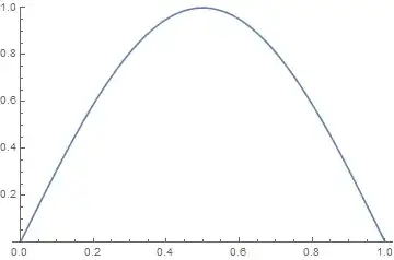
tp = Table[
   Plot[Evaluate[u[x, t, 200]], {x, 0, 1}, PlotRange -> {0, 1}], {t,
    0, .2, .005}];
ListAnimate[tp]
Range[42]doesn't give the same result asListPlot[{1,2}]. What is it that you really are doing? – corey979 Jun 22 '18 at 19:08x==0is indeed equivalent toDerivative[1,0][u][0,t] == 0, how did you code it? Please add the complete code sample. Also, notice your i.c. is inconsistent with b.c., so you'll face the problem mentioned here if you're not using"FiniteElement"method for spatial discretization. – xzczd Jun 23 '18 at 04:24