Inconsistent of initial and boundary condition in 1D PDE

Question

I am now dealing with the 1D PDE with periodic boundary condition given by the following:

$$ \partial_{t}u(t,x) = \partial_{x}u(t,x). \quad \text{with}\quad u(0,x)=\frac{1}{\sqrt{2\pi}}e^{-(x-\pi/4)^2/2}\quad u(t,-\pi)=u(t,\pi) $$

ufun = NDSolveValue[{\!\(
\*SubscriptBox[\(\[PartialD]\), \(t\)]\(u[t, \[Theta]]\)\) + \!\(
\*SubscriptBox[\(\[PartialD]\), \(\[Theta]\)]\(u[t, \[Theta]]\)\) == 
 0, u[0, \[Theta]] == Exp[-(\[Theta] - \[Pi]/4)^2], 
u[t, -\[Pi]] == u[t, \[Pi]]}, 
u, {t, 0, 0.1, 20}, {\[Theta], -\[Pi], \[Pi]}, 
Method -> {"MethodOfLines", 
 "SpatialDiscretization" -> {"TensorProductGrid", 
   "MinPoints" -> 200}}, PrecisionGoal -> 1];

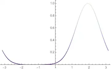
plots = Table[Plot[ufun[t, \[Theta]], {\[Theta], -\[Pi], \[Pi]},PlotRange -> {0, 1}, ColorFunction -> "LakeColors"], {t, 0, 
20, .1}];
ListAnimate[plots]

Although there is no error, the solution is not expected.

I have tried the solution here 2D Heat equation: inconsistent boundary and initial conditions.

 Method -> {"MethodOfLines", 
           "SpatialDiscretization" -> {"TensorProductGrid", "MinPoints" -> 20}}

It seems doesn't work. Any suggestion?

How about using "SpatialDiscretization" -> {"TensorProductGrid", "MinPoints" -> 200, "MaxPoints" -> 200}? That fixed it for me. Also, is PrecisionGoal -> 1 necessary? — Chris K, Aug 15 '18 at 17:20
@ChrisK It works! But I still didn't get it how does the these mesh affect the stability and why mathematica does not do these automatically? — Bob Lin, Aug 15 '18 at 17:47
I can't say for sure, but when I run your code it gives a warning Using maximum number of grid points 10000. Such a fine mesh size may mean that time steps need to be quite small to satisfy the Courant condition. I suppose numerically solving PDEs is a hard problem for Mathematica to make the right decisions on, so sometimes the user has to make the appropriate choice of numerical parameters. — Chris K, Aug 15 '18 at 17:58
BTW, welcome to Mathematica.SE! I suggest the following:

As you receive help, try to give it too, by answering questions in your area of expertise.

Take the [tour] and check the faqs!

When you see good questions and answers, vote them up by clicking the gray triangles, because the credibility of the system is based on the reputation gained by users sharing their knowledge.

Also, please remember to accept the answer, if any, that solves your problem, by clicking the checkmark sign! — Chris K, Aug 15 '18 at 17:59
Thanks for answering! I am wondering if there is a way to adaptively adjust the mesh to save memory and time (in 2D problem). — Bob Lin, Aug 15 '18 at 18:04
Sorry, I don't know about that. You might open another question on it if the 2D problem actually turns out to be problematic. — Chris K, Aug 15 '18 at 18:15
The time step of PDE solver is adaptive, but the spatial step is not (at least now). You can refer to tutorial/NDSolveMethodOfLines for more information — xzczd, Aug 16 '18 at 06:53
@xzczd Thanks! Btw, I am wondering if the unbounded transport equation can be solved by NDSolve perfectly or not? Do you think specifying a periodic boundary condition at some far away point like x=100 & -100 can mimic an unbounded problem? — Bob Lin, Aug 16 '18 at 08:12
To solve unbounded problem numerically, as you've noticed, artificial b.c. is often needed, but I never found material about artificial b.c. for transport equation. (This is a related post, don't miss the links there. ) The reason might be that, the analytic solution for transport equation is known and very simple. So I think it's better to solve transport equation analytically. — xzczd, Aug 16 '18 at 08:43
@xzczd Yes, you are right. Dsolve always treats this problem well. However, when I run into 2D problem (link), it seems to be inevitable to deal with this problem numerically like convection-dominated problem. — Bob Lin, Aug 16 '18 at 08:52

score 1 · Accepted Answer · answered Aug 17 '18 at 14:25

As I commented above, without setting "MaxPoints", NDSolve uses 10000 grid points, which makes it hard to solve, maybe due to the Courant condition. Adding "MaxPoints"->200 fixes it. I also removed PrecisionGoal->1 and changed the t range specification in NDSolve.

ufun = NDSolveValue[{
  D[u[t, θ] , t] + D[u[t, θ], θ] == 0, 
  u[0, θ] == Exp[-(θ - π/4)^2], 
  u[t, -π] == u[t, π]}, 
  u, {t, 0, 20}, {θ, -π, π}, 
  Method -> {"MethodOfLines", "SpatialDiscretization" -> {"TensorProductGrid", 
    "MinPoints" -> 200, "MaxPoints" -> 200}}];
Plot[ufun[20, θ], {θ, -π, π}, ColorFunction -> "LakeColors"]

Mathematica graphics

Inconsistent of initial and boundary condition in 1D PDE

1 Answers1