Problem with high parameter values in ParametricPlot

Question

I tried to plot the following function as a Parametric Plot. When I include values for w up to 1 the plot looks fine, but I need this plot for values up to 100 or 1000.

z[w_, L_, re_, r1_, c1_, r2_, WoR_, WoT_, WoP_, c2_] = 
     I w L + 1/(1/(I w c1) + 1/r1) + re + 
      1/(1/(I w c2) + 1/r2 + 
         1/(WoR*Coth[(I*WoT* w)^WoP]/(I*WoT* w)^WoP))

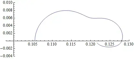
I want to have a Nyquist-Plot, so I plotted Real and Imaginary-Part with the following command:

ParametricPlot[{
   Re[z[w, 5.1867*10^(-7), 0.10549, 0.014394, 1.699, 
     0.0098142, 5.5173*10^(-7), 7.428*10^(-13), 0.19962, 0.085349]], 
   Im[z[w, 5.1867*10^(-7), 0.10549, 0.014394, 1.699, 
     0.0098142, 5.5173*10^(-7), 7.428*10^(-13), 0.19962, 
     0.085349]]}, {w, 0.000001, 1}, 
 PlotRange -> {{0.098, 0.13}, {-0.004, 0.01}}]

This works fine.

When I replace {w,0.000001,1} with {w,0.000001,1000} I get a weird plot.

Unfortunately I have no idea where the problem could be, so I posted the whole example. I think that there might be some numerical problem that is responsible for the weird edges in the second plot. For small w like 0.00001 the graph is not correct either, it should become negative.

Oh, I thought I needed that because Im does not work for symbolic expressions. But the plotting evaluates it... I will delete that. Does not solve the problem though. — Apatura, Jan 21 '13 at 15:12
For your reference, there is a new function NyquistPlot in Mathematica 9. — Silvia, Jan 21 '13 at 15:14
Does setting the option MaxRecursion -> Infinity for ParametricPlot solve your problem? — Silvia, Jan 21 '13 at 15:17
Welcome to Mathematica.SE and thank you for formatting your question properly. — Mr.Wizard, Jan 21 '13 at 15:18

score 4 · Accepted Answer · edited Apr 13 '17 at 12:55

4

I add MaxRecursion -> 15^(1),(2) to smooth out the line and Evaluated -> True^(3),(4) to speed evaluation. I also modified the code so that z is only called once and then passed to each Re and Im.

ParametricPlot[
 {Re@#, Im@#} & @ 
  z[w, 5.1867*10^(-7), 0.10549, 0.014394, 1.699, 0.0098142, 5.5173*10^(-7), 
   7.428*10^(-13), 0.19962, 0.085349],
 {w, 0.000001, 1000},
 PlotRange -> {{0.098, 0.13}, {-0.004, 0.01}},
 Evaluated -> True,
 MaxRecursion -> 15
]

Mathematica graphics

edited Apr 13 '17 at 12:55

Community

1

answered Jan 21 '13 at 15:12

Mr.Wizard

271,378
34
587
1,371

1

+1 btw I would prefer Through[{Re, Im}[...]]. – Silvia Jan 21 '13 at 15:20
@Silvia Thanks for the vote. I know some prefer that but as a fan of terse coding I like {Re@#, Im@#} & a little better. It's good you posted that though as I'm sure anyone who has not seen Through before will be glad. – Mr.Wizard Jan 21 '13 at 15:22
Yes, it's just a personal preference. Those #&@ things make me feel some kind of emotional instability :) – Silvia Jan 21 '13 at 15:30
@Silvia My code does sometimes have that effect on people. (See comments.) – Mr.Wizard Jan 21 '13 at 15:36
Now that really scared me!! – Silvia Jan 21 '13 at 16:24
Thanks a lot, @Mr.Wizard, that helps! But still the curve does not look the way I expected it. With another program (Zplot) I get completely different results. Is it possible that I have some numerical issues here with the cotangens hyperbolicus or something? – Apatura Jan 22 '13 at 13:39
@Apatura I'm sorry, I did not see your comment until now. If you have not already solved the problem please explain the difference and I will try to help. – Mr.Wizard Feb 06 '13 at 00:28

score 1 · Answer 2 · answered Mar 07 '13 at 22:59

It helps to parameterize the function so that the path is traced out at a fairly constant speed. Let's compute and plot the speed:

f[w_] := z[w, 5.1867*10^(-7), 0.10549, 0.014394, 1.699, 0.0098142, 
  5.5173*10^(-7), 7.428*10^(-13), 0.19962, 0.085349];
g[w_] := Evaluate @ D[f[w], w];
Plot[Norm[g[w]], {w, 10^-5, 10}, PlotRange -> Full, PlotStyle -> Thick]

Plot

Therein lies the problem: the speed undergoes a dramatic deceleration well before w even reaches $1$. Mathematica has trouble determining an appropriate "time" scale for constructing this plot. (Consequently, the usual expedients such as increasing the plot points or amount of recursive partitioning will have limited effects.)

One cure is to reparameterize the curve. In principle, any differentiable curve can be reparameterized to have constant speed: that's ideal. But we only need to roughly approximate this ideal, so let's just take a stab with a strongly nonlinear function, such as an exponential. It's easy enough to work out the effect on the speed, but let's just dumbly start over with w replaced by Exp[w], pretending we don't know how to differentiate:

g[w_] := Evaluate @ D[f[Exp[w]], w];
Plot[Norm[g[w]], {w, Log[.000001], Log[1000]}, PlotRange -> Full, PlotStyle -> Thick]

Replot

Now that is perfectly fine: there are swings in the speed, to be sure, but soon it settles down to a constant. Let's exploit this in the plot, replacing the old parameter w by Exp[w]:

ParametricPlot[
 Through[{Re[#] &, Im[#] &}[f[Exp[w]]]], {w, Log[10^-6], Log[10^6]}, 
 PlotRange -> {{0.098, 0.13}, {-0.004, 0.01}}, 
 PlotStyle -> Thick, ColorFunction -> Function[{x, y, t}, Hue[t]]]

Parametric plot

The hue provides a qualitative indication of the value of the corresponding parameter at each point, Exp[w]. The extremely low speeds at the outset have compressed the reds and oranges down almost to a point at the beginning (left) of the curve, but after that the graphic evolved just fine and Mathematica--guided by the typical speeds in this parameterization--has done a good job without any additional prompting.

Problem with high parameter values in ParametricPlot

2 Answers2

Linked