What algorithm does Plot use to determine abscissas?

Question

(I'm hoping this question is not hopelessly naive...)

My understanding is that Plot's strategy is to generate a list of abscissas, evaluate the argument expression at those abscissas, and from that point on behave pretty much like ListPlot with the list of abscissa-ordinate pairs as input. (More or less.)

Assuming that the sketch above is not fantastically off-base, what algorithm does Plot use to compute the list of abscissas to use?

@belisarius: interesting trick, thanks, but I confess that I don't feel much more capable of guessing Mathematica's algorithm for generating the mesh than I was before... — kjo, Jan 22 '13 at 19:48
Mma algorithms are usually proprietary (except when they disclose them explicitly) and usually not easy to guess from the behavior — Dr. belisarius, Jan 22 '13 at 19:51
@belisarius: Yeah, that's what I was alluding to with my opening parenthetical remark... Your comment basically tells me that, yep, my question was pretty naive... I guess I was hoping to find something like "Mathematica's algorithm is based on a fourth-order Craske-Trump adaptive bisection algorithm, but it has been enhanced with many proprietary modifications..." — kjo, Jan 22 '13 at 19:58
a more interesting varient on belisarius suggestion: ListPlot[Reap[Plot[Sow[x]; 1/(x - .5)^2, {x, 0, 1}]][[2, 1]]]. You can see that there is an adaptive curvitue based algorithm. Oddly it seems to never eval at the lower bound.. — george2079, Jan 22 '13 at 22:11
Is your question answered by the posts linked here?: http://mathematica.stackexchange.com/a/11142/121 — Mr.Wizard, Jan 22 '13 at 22:34
@Mr.Wizard: That link leads to quite a lode of insight on Plot's ways... Thanks! — kjo, Jan 23 '13 at 01:45

score 10 · Accepted Answer · answered Jan 22 '13 at 22:32

This doesn't really answer the question, but might help you with your investigations...

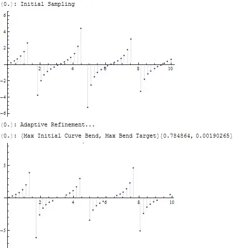
By setting the system option "VisualizationOptions" -> {"Verbose" -> True} you get all sorts of information printed about the plotting process. The code below intersperses that output with the actual sampled points (shown as ListPlots), showing the initial sampling and multiple refinement steps. There are numerical parameters associated with the refinement steps - they mean nothing to me but perhaps an expert could infer something about the algorithm.

plotinfo[func_, {from_, to_}] := Module[{a, f, g},
  SetSystemOptions["VisualizationOptions" -> {"Verbose" -> True}];
  a = SplitBy[Reap[Block[{Print = Sow[f[##]] &},
       Plot[func[x], {x, from, to}, EvaluationMonitor :>
         Sow[g[{x, func[x]}]]]]][[2, 1]], Head];
  SetSystemOptions["VisualizationOptions" -> {"Verbose" -> False}];
  a[[2 ;; -1 ;; 2]] = f@ListPlot[#, Filling -> Axis] & /@ a[[2 ;; -1 ;; 2, All, 1]];
  a /. f -> Print;]

The arguments are a function to plot and a range, e.g.

plotinfo[Tan, {0, 10}]

This is just a snippet of the full output:

enter image description here

Thanks! This was a beautiful answer. – kjo Aug 23 '13 at 11:48 — kjo, Aug 23 '13 at 11:48

What algorithm does Plot use to determine abscissas?

1 Answers1