How do I plot a solution of a differential equation?

Question

I am having trouble generating a plot for a solution to my differential equations. I always end up with just blank axes.

Clear["Global`*"] 
Remove["Global`*"]
m x''[t] == -k m x'[t];
m y''[t] == -k m y'[t] - m g;
U == v Cos[\[Theta]];
V == v Sin[\[Theta]];
soln = DSolve[{m x''[t] == -k m x'[t], m y''[t] == -k m y'[t] - m g, 
  x[0] == 0, y[0] == 0, x'[0] == U, y'[0] == V}, {x[t], y[t]}, 
 t][[1]] // Simplify;
soln
ParametricPlot[{x[t], y[t]}, {t, 0, 5}]

The solution comes out fine but the graph always comes out blank. I'm sure I'm making some rookie mistake somewhere and would appreciate if someone can point it out.

You can change ParametricPlot[{x[t], y[t]} /. soln, ...] and in order to get a plot you need to specify numerical values for your parameters. — b.gates.you.know.what, Jan 30 '13 at 09:10
My answer to an unrelated question gives an example of plotting solutions to NDSolve. — whuber, Jan 30 '13 at 15:26
Clear then Remove is redundant. Clear will remove all rules associated with a symbol, but the symbol remains known. Remove does that and removes the symbol from the "known" symbols list. Personally, I use Clear, and sometimes ClearAll, if I've set Attributes or attached Messages to the symbol, and reserve Remove for when I have to deal with shadowing. — rcollyer, Jan 30 '13 at 15:27
(cont'd) I also set each notebook to have its own Context, so that multiple notebooks do not conflict with each other. — rcollyer, Jan 30 '13 at 15:29

score 7 · Answer 1 · answered Jan 30 '13 at 09:30

In order plot your solution you have to replace all parameters with explicit values. One possible way is to use Manipulate.

m x''[t] == -k m x'[t];
m y''[t] == -k m y'[t] - m g;
U == v Cos[\[Theta]];
V == v Sin[\[Theta]];
soln = DSolve[{m x''[t] == -k m x'[t], m y''[t] == -k m y'[t] - m g, 
  x[0] == 0, y[0] == 0, x'[0] == U, y'[0] == V}, {x[t], y[t]}, 
 t][[1]] // Simplify;

With[{expr = {x[t], y[t]} /. soln},
 Manipulate[
  ParametricPlot[expr, {t, 0, 5}, PlotRange -> {{0, 10}, {-5, 5}}],
  {{k, 1}, .1, 5},
  {{g, 3}, 1, 10},
  {{U, 6}, 2, 10},
  {V, 5, 10}
  ]
 ]

Mathematica graphics

score 6 · Answer 2 · edited Jan 30 '13 at 17:17

I believe the main issue for you is that Mathematica does not know what x[t] and y[t] are in your ParametricPlot command. An excellent way to solve this is by using ReplaceAll (a.k.a. /.) with the Rules already included in the solution produced by DSolve.
Ensure that your parameters (e.g. U and V) are assigned values with Set (=); do not use Equal (==) here, which is an operator used to define equations and do logical comparisons of two expressions.
Assign values (using Set) to all of your parameters, as mentioned by user halirutan.

I propose the following improved code:

Clear["Global`*"]
m = k = v = θ = g = 1;
m x''[t] == -k m x'[t];
m y''[t] == -k m y'[t] - m g;
U = v Cos[θ];
V = v Sin[θ];
soln = DSolve[{m x''[t] == -k m x'[t], m y''[t] == -k m y'[t] - m g, 
x[0] == 0, y[0] == 0, x'[0] == U, y'[0] == V}, {x[t], y[t]}, t][[1]];
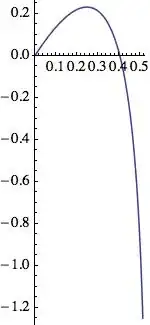
ParametricPlot[{x[t], y[t]} /. soln, {t, 0, 3}]

enter image description here

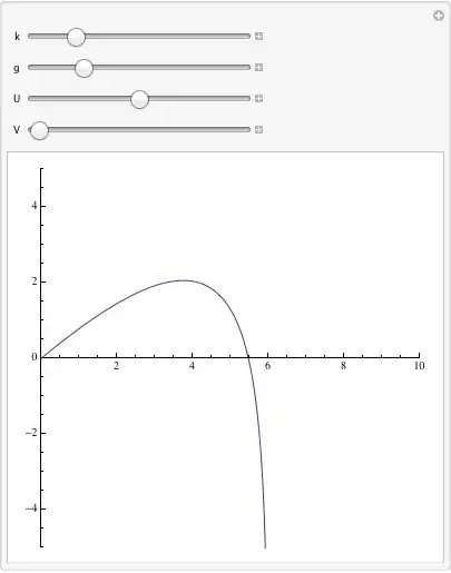
As a further example, I've included a direction field and a parametric plot of a specific solution for a different, first-order differential equation. The specific solution corresponds to a single value (in this case C[1] = 0) for the constant of integration which is in the general solution.

soln=DSolve[y'[x]==(x^2)/(1-y[x]^2),y[x],x];
plotone=ParametricPlot[{x,y[x]/.soln[[1]]/.C[1]->0},{x,-10,10}, PlotStyle->{Red, Thickness[0.01]}];
plottwo=StreamPlot[{(1 - y^2),x^2},{x,-10,10}, {y,-10,10}, VectorScale->.2, StreamStyle-> Blue];
Show[plottwo,plotone]

enter image description here

How do I plot a solution of a differential equation?

2 Answers2

Linked

Related